What is an image?
Basically, a digital image is an array of pixels.
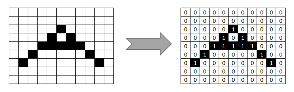
A binary image is nothing but a black and white image, in which each pixel will be either 1 or 0.
Morphological Operations:
Morphological operations are operations made on binary images based on mathematical concepts. These operations are useful in enhancing the images, detect edges of the objects in a image, remove unwanted or irrelevant noise pixels from the image and in partitioning the images to locate objects (Segmentation) and to identify it.
The most basic Morphological Operations are Erosion and Dilation.
Erosion and Dilation takes two inputs.
- Image Element
- Structuring Element
Image Element is the input image in which the Morphological Operations are applied.
What is a Structuring Element?
Structural Element is a matrix, usually small and simple. This element is used to observe the image element and identifies the matching pixels of the image (mathematically, hits or misses).
The morphological operations will be done based on the perfect match or partial match.
Analogy:
You can imagine that you are looking for a particular car in a car showroom. You will have the car design in your mind and verify whether it matches with any of the cars in the showroom. You may some time need the exact same car or sometimes the similar one with minor modifications are fine. The desired car you have in your mind is the Structuring Element here. The showroom is the Image you analyze.
So, the desired shape can be in 2D or 3D. If your input is a 2D Image Element, then the 2D structuring element is used. 3D Structuring Elements are used in 3D image datasets such as images obtained from a Magnetic Resonance Imaging (MRI) or Computed Tomography (CT) etc.
Image by Author
Thus, to construct a structuring Element, we need 2 properties. Shape and Size.
The usual size is of 3 X 3 or 5 X 5 or 21 X 21.
However, adjusting this shape will provide different results.
In this article, we will discuss about only the 2D images and 2D structuring elements.
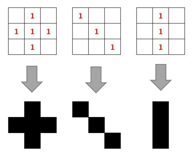
Usually, for basic Morphological operations such as Erosion & Dilation, this Element contains only 1s in a matrix which forms a shape of the structuring element.
A structuring element can be of any shape formed by 1s in a matrix. It can be a circle, square, rectangle, a cross or even a straight line. The entries in the matrix which is not the part of the structuring element can be left blank.
However, programmatically, as we cannot create a NumPy array of empty spaces, we represent these entries as 0. But these entries will not be counted when doing Erosion or Dilation.

Mathematically, 0 is also a number. As a structuring element does not always need to be 1s for other complex morphological operations, sometimes 0 also contribute to the shape of the Structuring Element.
Origin:
In most cases, the origin of the structuring element will be the centre entry. This can also be changed based on the shape or requirement.
The structuring element will slide over(convolute) the image based on the origin. This concept will be explained in detail in Erosion and Dilation.
If you are also learning or already know Computer Vision, this Structuring Element is the Kernel which convolutes over the image.
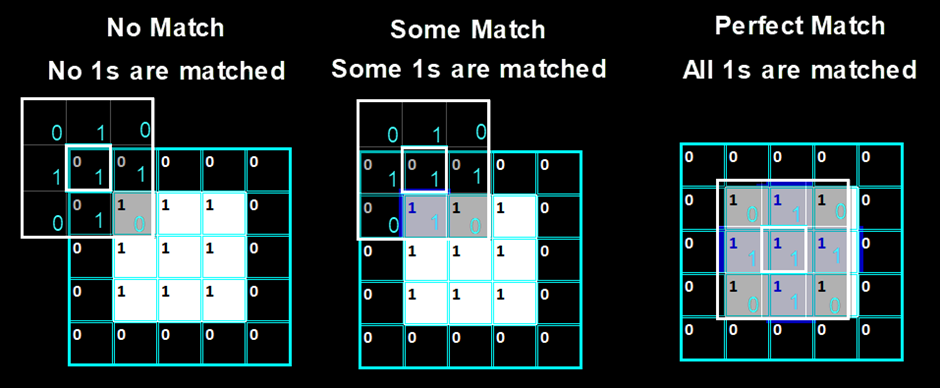
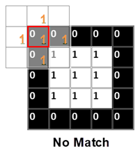
What is a Perfect Match, Some Match & No Match?
In the Erosion & Dilation process, the structuring element’s origin will stick over the image element, slide over it and the match will be verified.
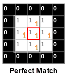
When the structuring element is placed on top of the image element, if all the 1s of the structuring element has a matching 1s in the Image element of the corresponding entry, then it is a Perfect Match.
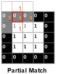
If some of the 1s of the Structuring Element has matching 1s in image, but not all the 1s, then it is Some Match.
If no 1s are matched with the image, then it is No Match.
These 3 concepts will be used in Erosion & Dilation operations.
Erosion:
Erosion is one of the most useful and simple morphological operation in digital image processing.
As its name means, erosion takes away the pixels lies in the borders of an object in the image or it takes away the irrelevant shape details in the objects.
In other words, Erosion shrinks the images.
We can also say that Erosion decreases the white area and increases the black area of a binary image. i.e., W ↓ B ↑
Mathematically, lets consider the white pixels as 1 and black pixels as 0.
As Erosion decreases the white pixels, we can denote erosion as ⊖.
A erosion B is A ⊖ B (Minus symbol enclosed in circle)
How to do erosion in a digital image?
To erode the image, the structuring element’s origin will stick over the image element and slide over the image element and the match will be verified.
Based on the erosion rules, all 1s of the Structuring Element will be verified for match with the Image Element entries.
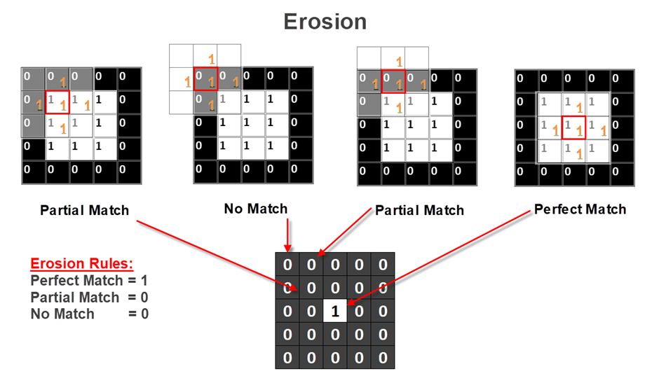
Erosion Rules:
| If all 1s are in… | The result will be… |
| Perfect Match | 1 |
| Some (Partial) Match | 0 |
| No Match | 0 |
Erosion Sample:

Erosion Process:
In the erosion of first and fifth entry in first row, there is no match of 1s. So the result will be 0.
In the second, third, fourth entries of first row, there is a partial match of bottom 1 of the structuring element. But Erosion will result 0 for Partial Match of 1s. So the result will be 0.
But when eroding the third row third entry, there will be a Perfect match of Top, Bottom, Left Right & Center 1s. So the result will be 1. As all other entries has no Perfect Match, other entries will be 0.
Erosion with OpenCV:
Lets take a binary image:
I have made the below image by just using Windows Paint and saved it as
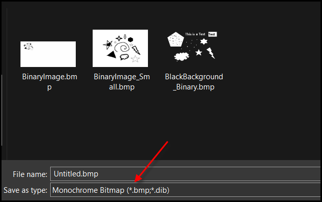
In this way we can get a binary image.
Read using OpenCV and view the image with matplotlib.pyplot:
import cv2
import matplotlib.pyplot as plt
import numpy as np
##Read image
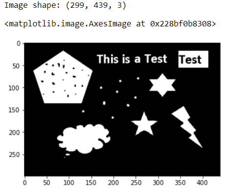
image_path="BlackBackground_Binary.bmp"
img=cv2.imread(image_path)
print("Image shape:", img.shape)
plt.imshow(img, cmap="gray")
Erosion using OpenCV erode function:
Lets try Erosion using a kernel of (filled) Square.
Kernel: [[1,1], [1,1], [1,1]]
# Kernel: a matrix of shape 3 X 3 with all entries as 1
kernel = np.ones((3,3), np.uint8)

img_erosion = cv2.erode(img, kernel, iterations=1)

plt.imshow(img_erosion, cmap="gray")
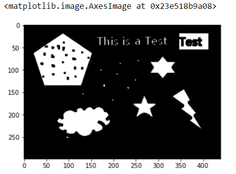
You can notice that the white pixels are decreased and black spaces are increased.
Below is another example of image with white background and black objects in foreground.
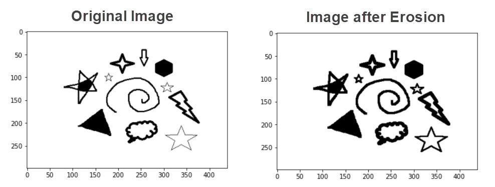
You can notice that the objects in image are thicker than original after Erosion. This is because the background color is white and after Erosion the white pixels are increased.
In the previous example, the objects were in white color and so the objects were shrunk.
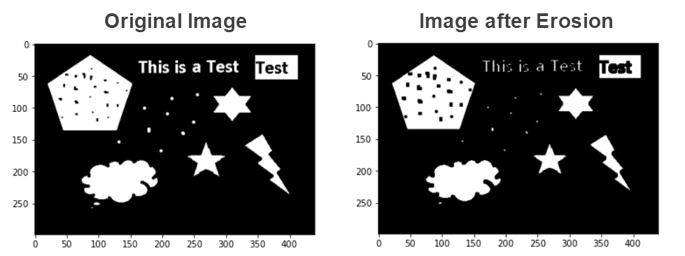
You can also notice that the white dots in the images were shrunk. If we increase the kernel (Structuring Element), then these dots will completely disappear from the image.
# Kernel: a matrix of shape 5 X 5 with all entries as 1
kernel = np.ones((5, 5), np.uint8)

img_erosion = cv2.erode(img, kernel, iterations=1)

plt.imshow(img_erosion, cmap="gray")
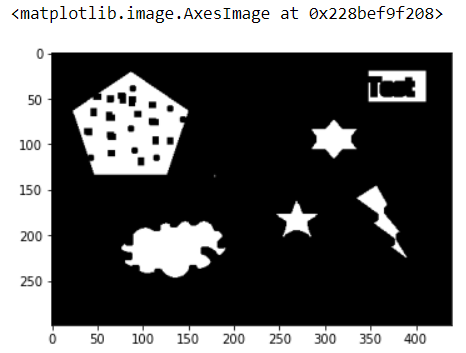
So by adjusting the structuring element, we can get different result.
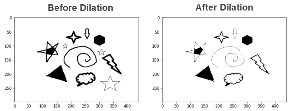
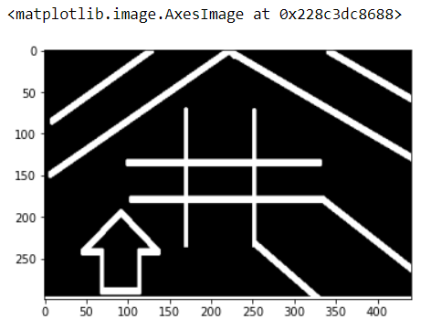
Lets erode the below image of lines.

The Kernel is a straight line.
# Kernel: Straight line
# Image: whiteBG_Lines.bmp
kernel_Slanting = [[0, 0, 1, 0, 0],
                   [0, 0, 1, 0, 0],
                   [0, 0, 1, 0, 0],
                   [0, 0, 1, 0, 0],
                   [0, 0, 1, 0, 0]]

kernel_Slanting = np.array(kernel_Slanting, np.uint8)

img_erosion = cv2.erode(img, kernel_Slanting, iterations=1)

plt.imshow(img_erosion, cmap="gray")

Notice that the 1s in Kernel is a straight line.
So the white spaces around all the shapes except straight lines are eroded.
That means the the Structuring element reduced the white pixels in all the objects except the matching shapes.
Dilation:
Opposite to Erosion, Dilation expands the image.
It increases the White pixels and decreases the black pixels. i.e., W ↑ B ↓
Mathematically, let’s consider the white pixels as 1 and black pixels as 0.
As Dilation increases the white pixels, we can denote erosion as ⊕.
A dilation B is A ⊕ B (Plus symbol enclosed in circle)
How to do dilation in a digital image?
As same as erosion, for Dilation, the structuring element’s origin will stick over the image element and slide over the image element and the match will be verified.
Based on the dilation rules, all 1s of the Structuring Element will be verified for match with the Image Element entries. If at least one 1 of the structuring element matches with the image element’s entry, then the result will be 1.
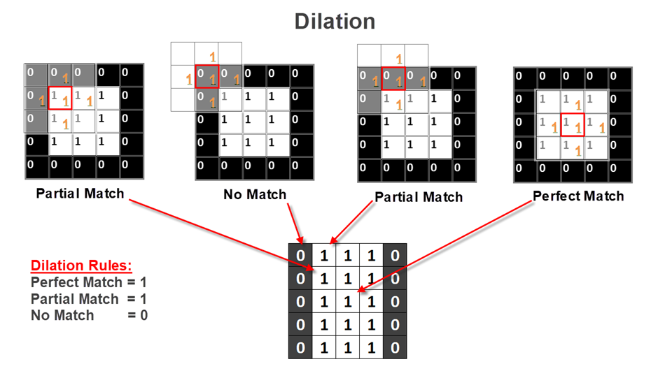
Dilation Rules:
| If all 1s are in… | The result will be… |
| Perfect Match | 1 |
| Some (Partial) Match | 1 |
| No Match | 0 |
In the below example, the structuring element is in Cross Shape. 1s in Top, Bottom, Left & Right.
If any of the 1s in these places matched then the result will be 1. 0 will be a result in less cases. Thus, the image will be expanded.
Dilation with OpenCV:
The original Image:
# Taking a matrix of size 5 as the kernel
kernel = np.ones((3,3), np.uint8)

img_dilation = cv2.dilate(img, kernel, iterations=1)

plt.imshow(img_dilation, cmap="gray")
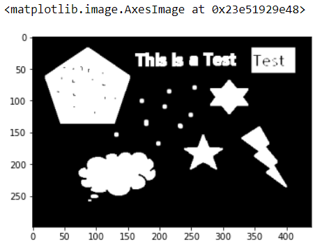
Notice that the white objects in image are expanded as dilation increases the white pixels.
Lets see the result in white BG example:
As the white pixels increased, the images the black objects were shrunk.
Lets see the result in another example where the shapes are filled with stripes.
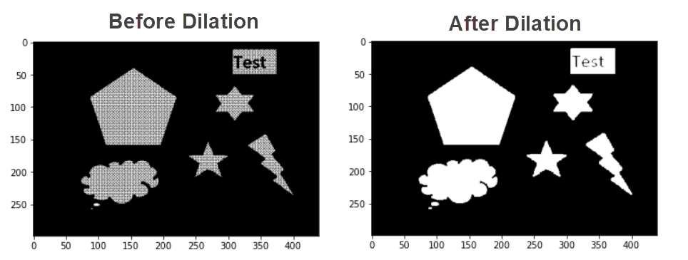
As the white pixels increased the objects became solid.
Using a Straight Line as Kernel:
Original object:

##Read image
image_path="whiteBG_Lines.bmp"
img=cv2.imread(image_path)

# Kernel: Straight line
# Image: whiteBG_Lines.bmp
kernel_Slanting = [[0, 0, 1, 0, 0],
                   [0, 0, 1, 0, 0],
                   [0, 0, 1, 0, 0],
                   [0, 0, 1, 0, 0],
                   [0, 0, 1, 0, 0]]

kernel_Slanting = np.array(kernel_Slanting, np.uint8)

img_dilation = cv2.dilate(img, kernel_Slanting, iterations=1)

plt.imshow(img_dilation, cmap="gray")
Notice that the objects that does not match with the structuring elements are dilated.
i.e. The white pixels near the non-matching elements are increased.
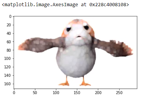
Lets test Erosion and Dilation in a color image:
import cv2
import numpy as np
import matplotlib.pyplot as plt

#Reading the input image
img = cv2.imread('bird.jpg')

#Convert the image to RGB
img = cv2.cvtColor(img, cv2.COLOR_BGR2RGB)

#Kernel: 5 X 5
kernel = np.ones((5,5), np.uint8)

#Erosion
img_erosion = cv2.erode(img, kernel, iterations=1)

#Dilation
img_dilation = cv2.dilate(img, kernel, iterations=1)

print("Original Image:")
plt.imshow(img)
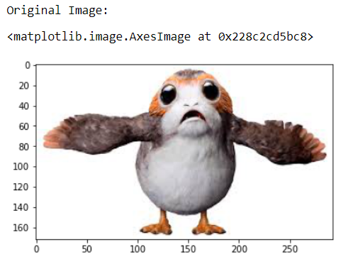
Image after Erosion:
plt.imshow(img_erosion)
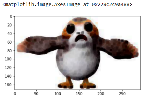
Image after Dilation:
plt.imshow(img_dilation)