
In this article, we will learn about tuning a Simple Multilayer Perceptron model using advanced Hyperparameters tuning techniques.
In our previous articles we have learned to construct basic Multi-layered Perceptron models for both Classification and Regression problems.
Artificial Neural Network Explained with an Regression Example
Deep Learning – Classification Example
Those are very simple construction of a model and explained with details.
Basic MLP:
We know that MLP is a simple/basic neural network for simple regression/classification tasks and which can achieved using Keras.
Lets take one more step and work with simple images.
MNIST Dataset:
The MNIST database is a collection of handwritten digits. It is one of the best dataset for new Neural Network learners and people who want to try different techniques in processing images.
This dataset has a training set of 60,000 examples, and a test set of 10,000 examples. It is a subset of a larger set available from NIST. The digits have been size-normalized and centered in a fixed-size image.
The official page of MNIST dataset is http://yann.lecun.com/exdb/mnist/.
Download the below files (Originally available in MNIST website):
train-images-idx3-ubyte.gz: training set images (9912422 bytes)
train-labels-idx1-ubyte.gz: training set labels (28881 bytes)
t10k-images-idx3-ubyte.gz: test set images (1648877 bytes)
t10k-labels-idx1-ubyte.gz: test set labels (4542 bytes)
Also this dataset is available in Keras library itself:
import matplotlib.pyplot as plt

from sklearn.model_selection import train_test_split
from keras.datasets import mnist
from keras.models import Sequential
from keras.utils.np_utils import to_categorical
Using TensorFlow backend.
Load Dataset:
(X_train, y_train), (X_test, y_test) = mnist.load_data()
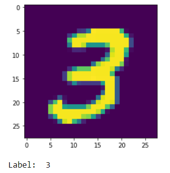
# show a number from the dataset
plt.imshow(X_train[7])
plt.show()
print('Label: ', y_train[7])
The numpy arrays X_train & X_test contains the images and y_train & y_test contains the labels.
Y value will be any number from 0 to 9.
X_train.shape, y_train.shape, X_test.shape, y_test.shape
((60000, 28, 28), (60000,), (10000, 28, 28), (10000,))
Here, notice that the image arrays X_train & X_test are in 3D array and labels are in 1D array.
Lets see the shape of a single image.
X_train[0].shape
(28, 28)
These handwritten digits images will originally look as shown below:

Okay, Lets get back to the model now.
Pre-Process X data:
We are going to make a model with Keras Sequential() Dense input layer.
As we know a black & white image is 2 Dimensional. A color image will have another dimension Channel. So it is 3D.
The Dense layer will only be applied on last axis of the image. For example, the image is of 2D say (dim_1, dim_2) then the Dense layer will be applied only on deim_2.
If the image is of 3D say (dim_1, dim_2, dim_3), then the dense layer will be applied only on dim_3.
So if we send the image as it is to the Dense layer, the last axis dim_2/dim_3 only be taken in account and the features will be considered in the model (i.e. weights will be assigned only in last axis).
To make the Dense layer to work on entire image without missing any features, we just flatten the image (numpy array) to single dimensional.
# To Flatten the image, reshaping X data: (n, 28, 28) => (n, 784)
# n => number of images. The actual size of a single image is (28, 28)
X_train = X_train.reshape((X_train.shape[0], -1))
X_test = X_test.reshape((X_test.shape[0], -1))
In this experiment, we only use the 33% of data to avoid complexity of execution.
X_train, _ , y_train, _ = train_test_split(X_train, y_train, test_size = 0.67, random_state = 7)
Pre-Process Y data:
If the output is a binary classification, then the number of nodes in output layer is one.
If the output is a multi-class classification, then the number of nodes in output layer should be the number of classes.
In our example, the label data is a number. But the output layer needs to fire any one value from 0 to 9. So we have to construct an output layer of 10 nodes.
If the model predicts the image as number “2”, then the output layer should fire the node which is allocated for “2”. i.e. it will result “1”. All other nodes should be 0. So, the output array will be [0 0 1 0 0 0 0 0 0 0].
To change the label values to an array of 10 binary values, we can use the one-hot encoding on the target value.
y_train = to_categorical(y_train)
y_test = to_categorical(y_test)
print(X_train.shape, X_test.shape, y_train.shape, y_test.shape)
(19800, 784) (10000, 784) (19800, 10) (10000, 10)
Basic MLP model using Keras:
Naïve MLP model:
from keras.models import Sequential
from keras.layers import Activation, Dense
from keras import optimizers
model = Sequential()

model.add(Dense(50, input_shape = (784, )))
model.add(Activation('sigmoid'))
model.add(Dense(50))
model.add(Activation('sigmoid'))
model.add(Dense(50))
model.add(Activation('sigmoid'))
model.add(Dense(50))
model.add(Activation('sigmoid'))
model.add(Dense(10))
model.add(Activation('softmax'))
We use the stochastic gradient descent optimizer here and compile the model with loss function “categorical_crossentropy” as it is a classification model.
sgd = optimizers.SGD(lr = 0.001)
model.compile(optimizer = sgd, loss = 'categorical_crossentropy', metrics = ['accuracy'])
Fit the model with the batch size of 256.
validation_split = 0.3: internally split 30% of data as a validation dataset and validate the model while training itself.
verbose is 0: Less log while fitting the model.
history = model.fit(X_train, y_train, batch_size = 256, validation_split = 0.3, epochs = 100, verbose = 0)
plt.plot(history.history['acc'])
plt.plot(history.history['val_acc'])
plt.legend(['training', 'validation'], loc = 'upper left')
plt.show()
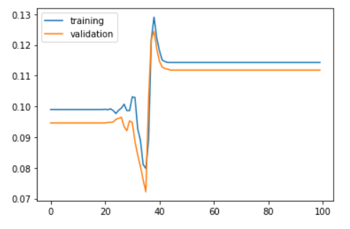
results = model.evaluate(X_test, y_test)
7872/10000 [======================>.......] - ETA: 0s
print('Test accuracy: ', results[1])
Test accuracy: 0.1135
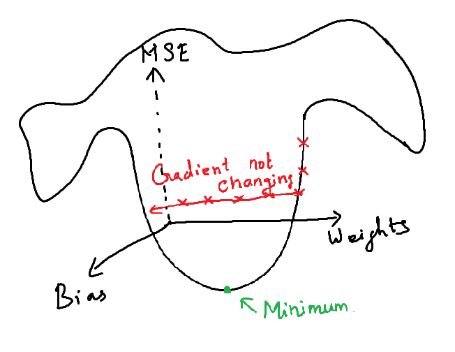
What is a Vanishing Gradient Problem?
In the above model, the test accuracy is very low. This is because the accuracy did not change after around 45th epoch. After this, the model provides same accuracy. i.e. The model did not learn anything after the 45th epoch.
The loss value was not reduced after the 45th iteration. This happens as the gradient value doesn’t change after certain iterations and this will no longer converge to the optimum value as there is no change in the gradient.
i.e., At each epoch, the weights will be adjusted in the back propagation. At each epoch, the gradients become smaller and reaches 0. Once, the gradients become 0, there will be no change in the weights. The weights remain same in all the remaining epochs. When this 0 Gradient happens in middle of the network (i.e., deep inside the network), the gradient descent will never converges to the optimum.
This issue is called vanishing gradient problem.
What is an Exploding Gradient Problem?
In some other cases, when all the neurons produce high positive values or when all the neurons produce very low values together, the loss value of the next iteration value will also have high variance from the previous iteration’s loss value. This will result in an unstable network and the there will be no learning.
There is a possibility of weights become NaN when the it becomes very large in further computations and so it will never converge. This problem is called Exploding Gradient problem.
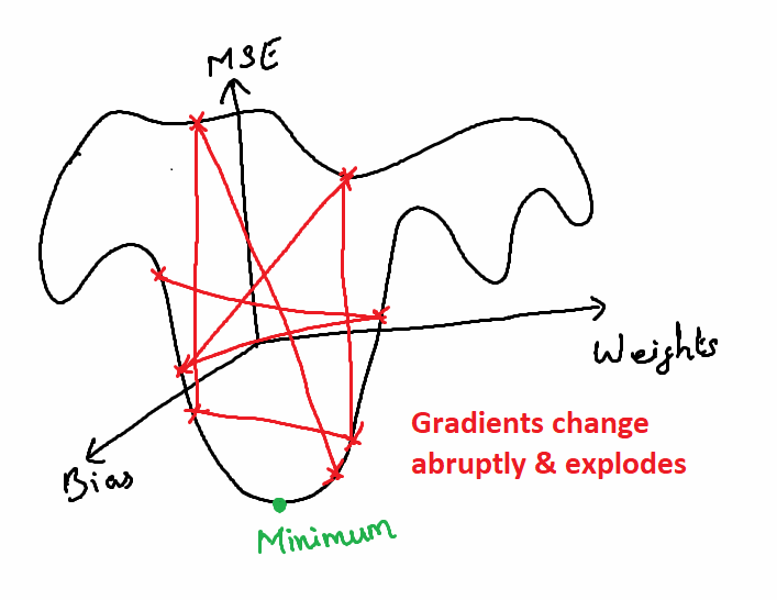
Deep learning was abandoned for long time after its discovery due to this problem.
This problem has been solved after the discovery of the below techniques:
- Weight Initialization
- Nonlinearity (Activation function)
- Optimizers
- Batch Normalization
- Dropout (Regularization)
Hyperparameter Tuning Techniques:
1. Weight Initialization
In the previous experiment, the model faced vanishing gradient problem and so there was no improvement after 45th epoch.
How to resolve vanishing gradient problem?
When the weights are assigned to keras layers, a scheme will be followed.
By default, the Dense layer will use “glorot_uniform” as default kernel initializer when no initializers are mentioned explicitly in dense layer. Dense layer documentation: https://keras.io/api/layers/core_layers/dense/
The weights are an important parameter of the model, which will be optimized to get a global minimum for better accuracy.
By adjusting the weight initialization scheme, the model can be improved and vanishing gradient problem can be prevented up to some degree.
In the paper written by researchers Xavier Glorot, Antoine Bordes, and Yoshua Bengio, they proposed an initialization strategy with uniform distribution.
With the help of Normalization, the weights should be chosen such that “the mean of all weights is 0” with the standard deviation based on number of inputs and outputs.
This initialization’s implementation is provided in Keras in the name “he_normal” and it is called Xavier & He Initialization.
Keras also provides various types of initializers. We can find all of them here.
Using He_Normal Initializer:
# Create a function to generate and return models.
def mlp_model():
    model = Sequential()

    model.add(Dense(50, input_shape = (784, ), kernel_initializer='he_normal'))     # use he_normal initializer
    model.add(Activation('sigmoid'))
    model.add(Dense(50, kernel_initializer='he_normal'))                            # use he_normal initializer
    model.add(Activation('sigmoid'))
    model.add(Dense(50, kernel_initializer='he_normal'))                            # use he_normal initializer
    model.add(Activation('sigmoid'))
    model.add(Dense(50, kernel_initializer='he_normal'))                            # use he_normal initializer
    model.add(Activation('sigmoid'))
    model.add(Dense(10, kernel_initializer='he_normal'))                            # use he_normal initializer
    model.add(Activation('softmax'))

    sgd = optimizers.SGD(lr = 0.001)
    model.compile(optimizer = sgd, loss = 'categorical_crossentropy', metrics = ['accuracy'])

    return model
model = mlp_model()
history = model.fit(X_train, y_train, validation_split = 0.3, epochs = 100, verbose = 0)
plt.plot(history.history['acc'])
plt.plot(history.history['val_acc'])
plt.legend(['training', 'validation'], loc = 'upper left')
plt.show()
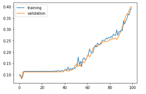
Now we can see that the accuracy is keep changing till 100th epoch even though the final accuracy is very less. However the model learns till the end.
results = model.evaluate(X_test, y_test)
9056/10000 [==========================>...] - ETA: 0s
print('Test accuracy: ', results[1])
Test accuracy: 0.4219
This solution is not enough.
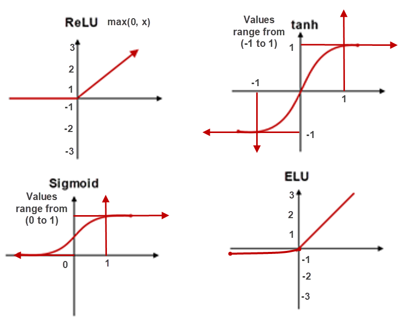
2. Activation function: (Nonlinearity)
Sigmoid functions has less saturation and the values will be ranged between 0 to +1. This will cause make training slower.
When the inputs to activation function is very large or very low, it will be changed to 1 or 0 respectively.
When the gradients are small, there is a high possibility to become 0 which is the vanishing gradient problem.
The best alternative of Sigmoid Function are ReLU, ELU, Leaky ReLU and Tanh.
These activation functions provide more saturation region than Sigmoid. However ReLU, ELU & Leaky ReLU provide higher saturation regions. These can mitigate Vanishing & Exploding Gradients problem.
For more information: https://devskrol.com/2020/11/08/how-neurons-work-and-how-artificial-neuron-mimics-neurons-in-human-brain/
Using ReLU &
In the below program, the ReLU function solves the vanishing gradient problem.
def mlp_model():
    model = Sequential()

    model.add(Dense(50, input_shape = (784, )))
    model.add(Activation('relu'))    # use relu
    model.add(Dense(50))
    model.add(Activation('relu'))    # use relu
    model.add(Dense(50))
    model.add(Activation('relu'))    # use relu
    model.add(Dense(50))
    model.add(Activation('relu'))    # use relu
    model.add(Dense(10))
    model.add(Activation('softmax'))

    sgd = optimizers.SGD(lr = 0.001)
    model.compile(optimizer = sgd, loss = 'categorical_crossentropy', metrics = ['accuracy'])

    return model
model = mlp_model()
history = model.fit(X_train, y_train, validation_split = 0.3, epochs = 100, verbose = 0)
plt.plot(history.history['acc'])
plt.plot(history.history['val_acc'])
plt.legend(['training', 'validation'], loc = 'upper left')
plt.show()
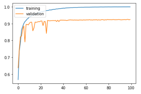
Now, training and validation accuracy improve instantaneously, but reach a plateau after around 30 epochs.
results = model.evaluate(X_test, y_test)
8512/10000 [========================>.....] - ETA: 0s
print('Test accuracy: ', results[1])
Test accuracy: 0.9188
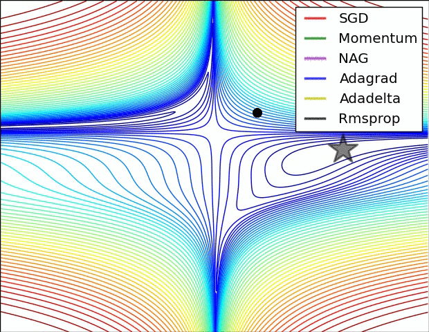
3. Optimizers
Optimizers are algorithms used to adjust the parameters (weights and learning rates) to reduce the loss/errors.
When discussing about Optimization and Optimizers, the first word comes to our mind is Gradient Descent. There are some major variations of Gradient Descents.
Batch Gradient Descent: Take the entire data set and computes the Gradient Descent.
i.e. For each epochs, the entire dataset is used in the calculation of MSE.
Stochastic Gradient Descent: Takes 1 random sample from the entire dataset.
Many variants of SGD are proposed and used nowadays. However all the optimizers has their own shortcomings. We can choose the optimizer based on the issue and usage.
One of the most popular ones are Adam (Adaptive Moment Estimation)
The below animation is an excellent illustration of comparison of optimizers made by Alec Radford. Unfortunately the Adam optimizer is not mentioned in this illustration.
Using Adam optimizer:
def mlp_model():
    model = Sequential()

    model.add(Dense(50, input_shape = (784, )))
    model.add(Activation('elu'))
    model.add(Dense(50))
    model.add(Activation('elu'))
    model.add(Dense(50))
    model.add(Activation('elu'))
    model.add(Dense(50))
    model.add(Activation('elu'))
    model.add(Dense(10))
    model.add(Activation('softmax'))

    adam = optimizers.Adam(lr = 0.001)                     # use Adam optimizer
    model.compile(optimizer = adam, loss = 'categorical_crossentropy', metrics = ['accuracy'])

    return model
model = mlp_model()
history = model.fit(X_train, y_train, validation_split = 0.3, epochs = 100, verbose = 0)
plt.plot(history.history['acc'])
plt.plot(history.history['val_acc'])
plt.legend(['training', 'validation'], loc = 'upper left')
plt.show()
Training and validation accuracy improve instantaneously, but reach plateau after around 50 epochs.
results = model.evaluate(X_test, y_test)
9792/10000 [============================>.] - ETA: 0s
print('Test accuracy: ', results[1])
Test accuracy: 0.9516
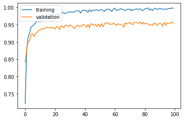
4. Batch Normalization
Another technique that was proposed to solve the vanishing gradient problem is batch Normalization.
Batch Normalization takes place immediate before the activation function of the layer. All the inputs of the current batch’s activation layer will be zero-centered and then passed to Activation functions.
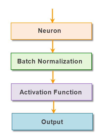
Batch normalization layer is usually inserted after dense/convolution and before nonlinearity:
from keras.layers import BatchNormalization
def mlp_model():
    model = Sequential()

    model.add(Dense(50, input_shape = (784, )))
    model.add(BatchNormalization())                    # Add Batchnorm layer before Activation
    model.add(Activation('elu'))
    model.add(Dense(50))
    model.add(BatchNormalization())                    # Add Batchnorm layer before Activation
    model.add(Activation('elu'))
    model.add(Dense(50))
    model.add(BatchNormalization())                    # Add Batchnorm layer before Activation
    model.add(Activation('elu'))
    model.add(Dense(50))
    model.add(BatchNormalization())                    # Add Batchnorm layer before Activation
    model.add(Activation('elu'))
    model.add(Dense(10))
    model.add(Activation('softmax'))

    adam = optimizers.Adam(lr = 0.001)
    model.compile(optimizer = adam, loss = 'categorical_crossentropy', metrics = ['accuracy'])

    return model
model = mlp_model()
history = model.fit(X_train, y_train, validation_split = 0.3, epochs = 100, verbose = 0)
plt.plot(history.history['acc'])
plt.plot(history.history['val_acc'])
plt.legend(['training', 'validation'], loc = 'upper left')
plt.show()
Training and validation accuracy improve consistently, but reach plateau after around 60 epochs:
results = model.evaluate(X_test, y_test)
9920/10000 [============================>.] - ETA: 0s
print('Test accuracy: ', results[1])
Test accuracy: 0.9643
5. Dropout (Regularization)
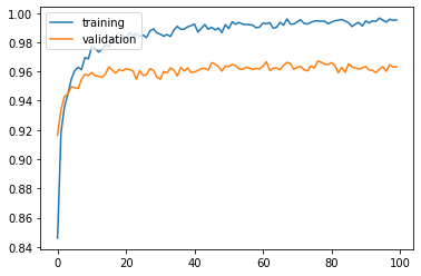
When the networks grow deeper, there is a chance of too much of learning the training data and overfit to it.
In the previous results, you can notice that the validation accuracy and training accuracies differ from each other. This is a sign of overfitting.
Dropout is a simple and powerful way to prevent overfitting. Some neurons will be randomly selected and dropped from the network in each layer.
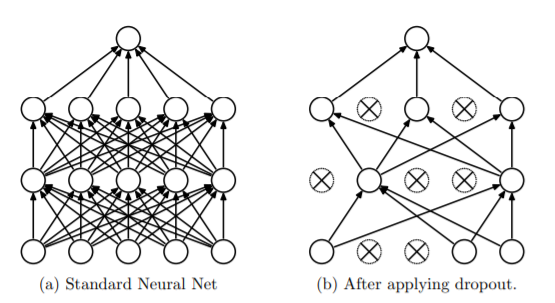
Right: After applying dropout to the network on the left.
Source: Journal on Dropout
from keras.layers import Dropout
def mlp_model():
    model = Sequential()

    model.add(Dense(50, input_shape = (784, )))
    model.add(Activation('elu'))
    model.add(Dropout(0.2))                        # Dropout layer after Activation
    model.add(Dense(50))
    model.add(Activation('elu'))
    model.add(Dropout(0.2))                        # Dropout layer after Activation
    model.add(Dense(50))
    model.add(Activation('elu'))
    model.add(Dropout(0.2))                        # Dropout layer after Activation
    model.add(Dense(50))
    model.add(Activation('elu'))
    model.add(Dropout(0.2))                         # Dropout layer after Activation
    model.add(Dense(10))
    model.add(Activation('softmax'))

    adam = optimizers.Adam(lr = 0.001)
    model.compile(optimizer = adam, loss = 'categorical_crossentropy', metrics = ['accuracy'])

    return model
model = mlp_model()
history = model.fit(X_train, y_train, validation_split = 0.3, epochs = 100, verbose = 1)
WARNING:tensorflow:From /anaconda3/lib/python3.6/site-packages/keras/backend/tensorflow_backend.py:2683: calling dropout (from tensorflow.python.ops.nn_ops) with keep_prob is deprecated and will be removed in a future version.
Instructions for updating:
Please use `rate` instead of `keep_prob`. Rate should be set to `rate = 1 – keep_prob`.
Train on 13860 samples, validate on 5940 samples
Epoch 1/100
13860/13860 [==============================] – 1s – loss: 11.7781 – acc: 0.2507 – val_loss: 8.8883 – val_acc: 0.4418
Epoch 2/100
13860/13860 [==============================] – 1s – loss: 8.1964 – acc: 0.4492 – val_loss: 4.0776 – val_acc: 0.5414
Epoch 3/100
13860/13860 [==============================] – 1s – loss: 1.9435 – acc: 0.4232 – val_loss: 1.3858 – val_acc: 0.5146
Epoch 4/100
13860/13860 [==============================] – 1s – loss: 1.4648 – acc: 0.5248 – val_loss: 1.0818 – val_acc: 0.6497
Epoch 5/100
13860/13860 [==============================] – 1s – loss: 1.2794 – acc: 0.5700 – val_loss: 1.0147 – val_acc: 0.6532
Epoch 6/100
13860/13860 [==============================] – 1s – loss: 1.1909 – acc: 0.6050 – val_loss: 0.8563 – val_acc: 0.7061
Epoch 7/100
13860/13860 [==============================] – 1s – loss: 1.0808 – acc: 0.6302 – val_loss: 0.9092 – val_acc: 0.7527
Epoch 8/100
13860/13860 [==============================] – 1s – loss: 0.9758 – acc: 0.6760 – val_loss: 0.6982 – val_acc: 0.7704
Epoch 9/100
13860/13860 [==============================] – 1s – loss: 0.8939 – acc: 0.6992 – val_loss: 0.6988 – val_acc: 0.7535
Epoch 10/100
13860/13860 [==============================] – 1s – loss: 0.8390 – acc: 0.7185 – val_loss: 0.6327 – val_acc: 0.8057
Epoch 11/100
13860/13860 [==============================] – 1s – loss: 0.8090 – acc: 0.7359 – val_loss: 0.5771 – val_acc: 0.8202
Epoch 12/100
13860/13860 [==============================] – 1s – loss: 0.7432 – acc: 0.7628 – val_loss: 0.5294 – val_acc: 0.8391
Epoch 13/100
13860/13860 [==============================] – 1s – loss: 0.7110 – acc: 0.7773 – val_loss: 0.5175 – val_acc: 0.8367
Epoch 14/100
13860/13860 [==============================] – 1s – loss: 0.6765 – acc: 0.7848 – val_loss: 0.5445 – val_acc: 0.8227
Epoch 15/100
13860/13860 [==============================] – 1s – loss: 0.6418 – acc: 0.8006 – val_loss: 0.4434 – val_acc: 0.8837
Epoch 16/100
13860/13860 [==============================] – 1s – loss: 0.5922 – acc: 0.8183 – val_loss: 0.4393 – val_acc: 0.8790
Epoch 17/100
13860/13860 [==============================] – 1s – loss: 0.5622 – acc: 0.8268 – val_loss: 0.4533 – val_acc: 0.8803
Epoch 18/100
13860/13860 [==============================] – 1s – loss: 0.5369 – acc: 0.8313 – val_loss: 0.3731 – val_acc: 0.8971
Epoch 19/100
13860/13860 [==============================] – 1s – loss: 0.5224 – acc: 0.8374 – val_loss: 0.3707 – val_acc: 0.8985
Epoch 20/100
13860/13860 [==============================] – 1s – loss: 0.5383 – acc: 0.8328 – val_loss: 0.3750 – val_acc: 0.9012
Epoch 21/100
13860/13860 [==============================] – 1s – loss: 0.5160 – acc: 0.8376 – val_loss: 0.3942 – val_acc: 0.8869
Epoch 22/100
13860/13860 [==============================] – 1s – loss: 0.4935 – acc: 0.8449 – val_loss: 0.3819 – val_acc: 0.8918
Epoch 23/100
13860/13860 [==============================] – 1s – loss: 0.5042 – acc: 0.8413 – val_loss: 0.3655 – val_acc: 0.9077
Epoch 24/100
13860/13860 [==============================] – 1s – loss: 0.4921 – acc: 0.8416 – val_loss: 0.3497 – val_acc: 0.9071
Epoch 25/100
13860/13860 [==============================] – 1s – loss: 0.4582 – acc: 0.8566 – val_loss: 0.3404 – val_acc: 0.9104
Epoch 26/100
13860/13860 [==============================] – 1s – loss: 0.4437 – acc: 0.8577 – val_loss: 0.3383 – val_acc: 0.91670
Epoch 27/100
13860/13860 [==============================] – 1s – loss: 0.4625 – acc: 0.8512 – val_loss: 0.3382 – val_acc: 0.9067
Epoch 28/100
13860/13860 [==============================] – 1s – loss: 0.4253 – acc: 0.8602 – val_loss: 0.3126 – val_acc: 0.9180
Epoch 29/100
13860/13860 [==============================] – 1s – loss: 0.4201 – acc: 0.8676 – val_loss: 0.3098 – val_acc: 0.9236
Epoch 30/100
13860/13860 [==============================] – 1s – loss: 0.4182 – acc: 0.8646 – val_loss: 0.2991 – val_acc: 0.9249
Epoch 31/100
13860/13860 [==============================] – 1s – loss: 0.4326 – acc: 0.8583 – val_loss: 0.3016 – val_acc: 0.9222
Epoch 32/100
13860/13860 [==============================] – 1s – loss: 0.4252 – acc: 0.8614 – val_loss: 0.3117 – val_acc: 0.9239
Epoch 33/100
13860/13860 [==============================] – 1s – loss: 0.4031 – acc: 0.8717 – val_loss: 0.2914 – val_acc: 0.9279
Epoch 34/100
13860/13860 [==============================] – 1s – loss: 0.3925 – acc: 0.8693 – val_loss: 0.2992 – val_acc: 0.9234
Epoch 35/100
13860/13860 [==============================] – 1s – loss: 0.4050 – acc: 0.8675 – val_loss: 0.2975 – val_acc: 0.9241
Epoch 36/100
13860/13860 [==============================] – 1s – loss: 0.3977 – acc: 0.8711 – val_loss: 0.3076 – val_acc: 0.9285
Epoch 37/100
13860/13860 [==============================] – 1s – loss: 0.3790 – acc: 0.8786 – val_loss: 0.2874 – val_acc: 0.9266
Epoch 38/100
13860/13860 [==============================] – 1s – loss: 0.3769 – acc: 0.8797 – val_loss: 0.2788 – val_acc: 0.9259
Epoch 39/100
13860/13860 [==============================] – 1s – loss: 0.3821 – acc: 0.8799 – val_loss: 0.2802 – val_acc: 0.9232
Epoch 40/100
13860/13860 [==============================] – 1s – loss: 0.3797 – acc: 0.8805 – val_loss: 0.2996 – val_acc: 0.9204
Epoch 41/100
13860/13860 [==============================] – 1s – loss: 0.3675 – acc: 0.8814 – val_loss: 0.2619 – val_acc: 0.9310
Epoch 42/100
13860/13860 [==============================] – 1s – loss: 0.3452 – acc: 0.8874 – val_loss: 0.2798 – val_acc: 0.9303
Epoch 43/100
13860/13860 [==============================] – 1s – loss: 0.3571 – acc: 0.8851 – val_loss: 0.3244 – val_acc: 0.9145
Epoch 44/100
13860/13860 [==============================] – 1s – loss: 0.3472 – acc: 0.8850 – val_loss: 0.2637 – val_acc: 0.9365
Epoch 45/100
13860/13860 [==============================] – 1s – loss: 0.3560 – acc: 0.8877 – val_loss: 0.2720 – val_acc: 0.9328
Epoch 46/100
13860/13860 [==============================] – 1s – loss: 0.3548 – acc: 0.8862 – val_loss: 0.2884 – val_acc: 0.9246
Epoch 47/100
13860/13860 [==============================] – 1s – loss: 0.3397 – acc: 0.8894 – val_loss: 0.3194 – val_acc: 0.9194
Epoch 48/100
13860/13860 [==============================] – 1s – loss: 0.3410 – acc: 0.8871 – val_loss: 0.2647 – val_acc: 0.9340
Epoch 49/100
13860/13860 [==============================] – 1s – loss: 0.3500 – acc: 0.8846 – val_loss: 0.2971 – val_acc: 0.9291
Epoch 50/100
13860/13860 [==============================] – 1s – loss: 0.3439 – acc: 0.8873 – val_loss: 0.3026 – val_acc: 0.9241
Epoch 51/100
13860/13860 [==============================] – 1s – loss: 0.3459 – acc: 0.8891 – val_loss: 0.2795 – val_acc: 0.9318
Epoch 52/100
13860/13860 [==============================] – 1s – loss: 0.3338 – acc: 0.8900 – val_loss: 0.2745 – val_acc: 0.9345
Epoch 53/100
13860/13860 [==============================] – 1s – loss: 0.3266 – acc: 0.8906 – val_loss: 0.2773 – val_acc: 0.9308
Epoch 54/100
13860/13860 [==============================] – 1s – loss: 0.3152 – acc: 0.9004 – val_loss: 0.2822 – val_acc: 0.9308
Epoch 55/100
13860/13860 [==============================] – 1s – loss: 0.3250 – acc: 0.8937 – val_loss: 0.2875 – val_acc: 0.9327
Epoch 56/100
13860/13860 [==============================] – 1s – loss: 0.3328 – acc: 0.8939 – val_loss: 0.2551 – val_acc: 0.9364
Epoch 57/100
13860/13860 [==============================] – 1s – loss: 0.3299 – acc: 0.8916 – val_loss: 0.2634 – val_acc: 0.9357
Epoch 58/100
13860/13860 [==============================] – 1s – loss: 0.3127 – acc: 0.8947 – val_loss: 0.2671 – val_acc: 0.9313
Epoch 59/100
13860/13860 [==============================] – 1s – loss: 0.2939 – acc: 0.9033 – val_loss: 0.2605 – val_acc: 0.9364
Epoch 60/100
13860/13860 [==============================] – 1s – loss: 0.2995 – acc: 0.9001 – val_loss: 0.2781 – val_acc: 0.9320
Epoch 61/100
13860/13860 [==============================] – 1s – loss: 0.3133 – acc: 0.8992 – val_loss: 0.2697 – val_acc: 0.9396
Epoch 62/100
13860/13860 [==============================] – 1s – loss: 0.3090 – acc: 0.8988 – val_loss: 0.2788 – val_acc: 0.9327
Epoch 63/100
13860/13860 [==============================] – 1s – loss: 0.3111 – acc: 0.8942 – val_loss: 0.2641 – val_acc: 0.9369
Epoch 64/100
13860/13860 [==============================] – 1s – loss: 0.3074 – acc: 0.8991 – val_loss: 0.2582 – val_acc: 0.9357
Epoch 65/100
13860/13860 [==============================] – 1s – loss: 0.3095 – acc: 0.8947 – val_loss: 0.2631 – val_acc: 0.9367
Epoch 66/100
13860/13860 [==============================] – 1s – loss: 0.3115 – acc: 0.8980 – val_loss: 0.2700 – val_acc: 0.9372
Epoch 67/100
13860/13860 [==============================] – 1s – loss: 0.3004 – acc: 0.8980 – val_loss: 0.2769 – val_acc: 0.9342
Epoch 68/100
13860/13860 [==============================] – 1s – loss: 0.2931 – acc: 0.9045 – val_loss: 0.2734 – val_acc: 0.9333
Epoch 69/100
13860/13860 [==============================] – 1s – loss: 0.3015 – acc: 0.8980 – val_loss: 0.2592 – val_acc: 0.9404
Epoch 70/100
13860/13860 [==============================] – 1s – loss: 0.2938 – acc: 0.9006 – val_loss: 0.2668 – val_acc: 0.9419
Epoch 71/100
13860/13860 [==============================] – 1s – loss: 0.2936 – acc: 0.9016 – val_loss: 0.2700 – val_acc: 0.9401
Epoch 72/100
13860/13860 [==============================] – 1s – loss: 0.3001 – acc: 0.9005 – val_loss: 0.2694 – val_acc: 0.9384
Epoch 73/100
13860/13860 [==============================] – 1s – loss: 0.2982 – acc: 0.9043 – val_loss: 0.2702 – val_acc: 0.9364
Epoch 74/100
13860/13860 [==============================] – 1s – loss: 0.2897 – acc: 0.9040 – val_loss: 0.2645 – val_acc: 0.9399
Epoch 75/100
13860/13860 [==============================] – 1s – loss: 0.2817 – acc: 0.9078 – val_loss: 0.2571 – val_acc: 0.9412
Epoch 76/100
13860/13860 [==============================] – 1s – loss: 0.2782 – acc: 0.9104 – val_loss: 0.2860 – val_acc: 0.9332
Epoch 77/100
13860/13860 [==============================] – 1s – loss: 0.2925 – acc: 0.9098 – val_loss: 0.2660 – val_acc: 0.9374
Epoch 78/100
13860/13860 [==============================] – 1s – loss: 0.2795 – acc: 0.9109 – val_loss: 0.2726 – val_acc: 0.9399
Epoch 79/100
13860/13860 [==============================] – 1s – loss: 0.2807 – acc: 0.9104 – val_loss: 0.2675 – val_acc: 0.9391
Epoch 80/100
13860/13860 [==============================] – 1s – loss: 0.2725 – acc: 0.9113 – val_loss: 0.2774 – val_acc: 0.9444
Epoch 81/100
13860/13860 [==============================] – 1s – loss: 0.2748 – acc: 0.9135 – val_loss: 0.2774 – val_acc: 0.9379
Epoch 82/100
13860/13860 [==============================] – 1s – loss: 0.2800 – acc: 0.9100 – val_loss: 0.3031 – val_acc: 0.9340
Epoch 83/100
13860/13860 [==============================] – 1s – loss: 0.2876 – acc: 0.9093 – val_loss: 0.2791 – val_acc: 0.9397
Epoch 84/100
13860/13860 [==============================] – 1s – loss: 0.2759 – acc: 0.9145 – val_loss: 0.2769 – val_acc: 0.9426
Epoch 85/100
13860/13860 [==============================] – 1s – loss: 0.2607 – acc: 0.9177 – val_loss: 0.2589 – val_acc: 0.9428
Epoch 86/100
13860/13860 [==============================] – 1s – loss: 0.2626 – acc: 0.9177 – val_loss: 0.2639 – val_acc: 0.9401
Epoch 87/100
13860/13860 [==============================] – 1s – loss: 0.2646 – acc: 0.9165 – val_loss: 0.2710 – val_acc: 0.9359
Epoch 88/100
13860/13860 [==============================] – 1s – loss: 0.2669 – acc: 0.9178 – val_loss: 0.2730 – val_acc: 0.9382
Epoch 89/100
13860/13860 [==============================] – 1s – loss: 0.2663 – acc: 0.9194 – val_loss: 0.2798 – val_acc: 0.9365
Epoch 90/100
13860/13860 [==============================] – 1s – loss: 0.2573 – acc: 0.9198 – val_loss: 0.2836 – val_acc: 0.9401
Epoch 91/100
13860/13860 [==============================] – 1s – loss: 0.2558 – acc: 0.9181 – val_loss: 0.2935 – val_acc: 0.9322
Epoch 92/100
13860/13860 [==============================] – 1s – loss: 0.2567 – acc: 0.9224 – val_loss: 0.2847 – val_acc: 0.9367
Epoch 93/100
13860/13860 [==============================] – 1s – loss: 0.2535 – acc: 0.9227 – val_loss: 0.3196 – val_acc: 0.9409
Epoch 94/100
13860/13860 [==============================] – 1s – loss: 0.2557 – acc: 0.9239 – val_loss: 0.2711 – val_acc: 0.9394
Epoch 95/100
13860/13860 [==============================] – 1s – loss: 0.2530 – acc: 0.9234 – val_loss: 0.2767 – val_acc: 0.9396
Epoch 96/100
13860/13860 [==============================] – 1s – loss: 0.2483 – acc: 0.9259 – val_loss: 0.2897 – val_acc: 0.9370
Epoch 97/100
13860/13860 [==============================] – 1s – loss: 0.2526 – acc: 0.9268 – val_loss: 0.2689 – val_acc: 0.9374
Epoch 98/100
13860/13860 [==============================] – 1s – loss: 0.2556 – acc: 0.9242 – val_loss: 0.2797 – val_acc: 0.9389
Epoch 99/100
13860/13860 [==============================] – 1s – loss: 0.2437 – acc: 0.9259 – val_loss: 0.2840 – val_acc: 0.9350
Epoch 100/100
13860/13860 [==============================] – 1s – loss: 0.2533 – acc: 0.9262 – val_loss: 0.2803 – val_acc: 0.9332
plt.plot(history.history['acc'])
plt.plot(history.history['val_acc'])
plt.legend(['training', 'validation'], loc = 'upper left')
plt.show()
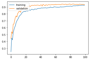
The validation and training results seems to be similar. Hence, applying dropout is one of the simple way to mitigate overfitting.
results = model.evaluate(X_test, y_test)
8640/10000 [========================>.....] - ETA: 0s
print('Test accuracy: ', results[1])
Test accuracy: 0.9309
Hyperparameter tuning cannot be done with a set of fixed steps. These are the ways of tuning the algorithm’s parameters to get the best from the algorithm.
So we can further make changes in the parameters, number of layers, number of nodes in each layer to get the best result.