Artificial Neural Network Explained with an Regression Example

In this article, we are going to discuss about the basics of Implementing a simple Artificial Neural Network (ANN).

It is recommended to know how Artificial Neurons mimic Neurons of human brain. Please read this article for easy understanding.
If you are excited to know about the history of ANN, please check this article.

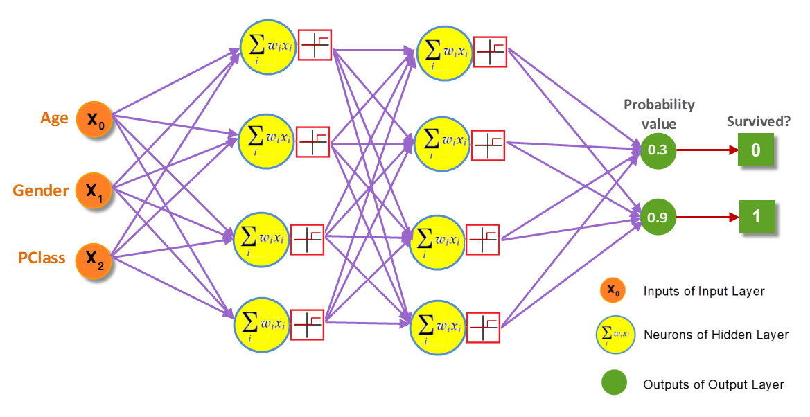
Architecture Of ANN:

1. Input Layer receives input:Input layer is a set of nodes which takes the input data as one per node.
   For a regression problem, if we are having 10 columns/features, then we need to set exactly 10 nodes in Input Layer.
2. Hidden Layers:An ANN can have one or more hidden layers. Each layer can have any number of Neurons.
   Each Neuron is a combination of an computational unit and an activation unit.
3. Output Layer:Each ANN has one Output Layer which provides the output of model.If the model is Regression, then the Output Layer will have only one Node. The output of this Node is the Y-Predicted value of the input given in Input Layer.If the target variable is a categorical data of two classes, then the Output Layer should have 2 Nodes and the activation function should be ‘Sigmoid’.If it is a multi-class classification, then the Output Layer should have Nodes exactly the same number of classes of the target variable. And the activation function should be ‘Softmax’.

   If the activation function is Sigmoid or Softmax, we will get the probability value from all the Nodes in the Output Layer. The index of the Highest Probability value is the output.

   To convert the Y value as categorical data,

   y_data = to_categorical(y_data)
   

4. Weights & Bias:Each connection mentioned in the picture is assigned with weight and bias. The weight value is initially assigned randomly and will be updated by the optimizers in each epochs. The Bias value is used to avoid the weights to become zero

APIs to construct ANN:

There are numerous APIs are available to construct ANN.

Most popular API is TensorFlow from Google. It is interfaced with Python & Numpy.

There are some other APIs that made on top of Tensorflow to make it more easy to use. One such

API is Keras. In this article we are going to use Keras.

Important Classes from Keras to Construct ANN:

1. The Squential() class helps to group the linear stack of layers. This class returns a model object that can be used to add more layers.

from keras.models import Sequential
model = Sequential()

2. The Dense() class implements a Layer.

It can be used in both input, hidden & output layers.

ANN with Regression:

A dense Node in Hidden Layer and Output Layer will get an Weight from each connection and calculate (Weight * input) + Bias. All the results from all the connections will be added together and given as output to the Neuron in Next Layer.

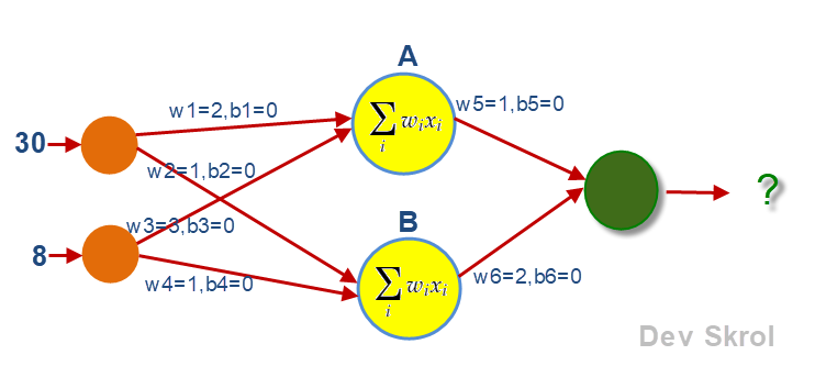
For example, If our data is having 2 features Age and Exp and its values are 30 & 8 and the Salary is 40,000, the features 30 & 8 will be given as input to the nodes of input layers.

As per the above picture, the weight and bias values will be assigned randomly.

The calculations in the Neurons:

A = (302 + 0) + (83 + 0) = 84

B = (301 + 0) + (81 + 0) = 38

Output = (841 + 0) + (382 + 0) = 160

160 is the output of the First Feed Forward process.

This value is not matching with the salary column value 40,000.

To get this output as 40,000, the weights will be updated in the Back Propagation process.

At this place, the specified Optimizer (Example: Gradient Descent, Adam etc) will take care of this process.

First the weights w5 & w6 will be updated. Then the next set of weights w1, w2, w3 & w4 will be updated.

This And then the feed forward will happen again for the next data.

Similarly the weights & biases will be updated for the remaining data and epochs.

from keras.layers import Dense

model = Sequential()

model.add(Dense(2, input_shape = (2,), activation= 'sigmoid'))
model.add(Dense(10, activation= 'sigmoid'))
model.add(Dense(10, activation= 'sigmoid'))
model.add(Dense(1))

Now the architecture of our Model is constructed.

We need to choose the right loss function and optimizer for Back Propagation.

from keras import optimizers

sgd = optimizers.SGD()

model.compile(optimizer = sgd, loss = 'mean_squared_error', metrics= ['mse', 'mae'])
model.summary()

Output:

Model: "sequential"
_________________________________________________________________
Layer (type)                 Output Shape              Param #   
=================================================================
dense (Dense)                (None, 20)                280       
_________________________________________________________________
dense_1 (Dense)              (None, 10)                210       
_________________________________________________________________
dense_2 (Dense)              (None, 10)                110       
_________________________________________________________________
dense_3 (Dense)              (None, 1)                 11        
=================================================================
Total params: 611
Trainable params: 611
Non-trainable params: 0
_________________________________________________________________

In the above summary, we can see the “Trainable params: 611” which means the weights and biases are totally 611 for the above mentioned network.

model.fit(X_train, Y_train, batch_size= 40, epochs=100, verbose= 0)
train_pred = model.predict(X_train)
test_pred = model.predict(X_test)

from sklearn.metrics import mean_squared_error, mean_absolute_error

print("Train Accuracy: ",mean_squared_error(Y_train, train_pred))
print("Test Accuracy: ",mean_squared_error(Y_test, test_pred))

Output:

Train Accuracy:  85.60549570539762
Test Accuracy:  86.0492232511959

Conclusion:

In this article, we have seen the Architecture of an Artificial Neural Network and how it works.
In the next article, we will see a complete Regression example.

Thank you for reading our article and hope you enjoyed it. 😊

Like to support? Just click the like button ❤️.

Happy Learning! 👩‍💻