5 Part series of most important Data Pre-Processing Techniques of Machine Learning:
- Part 5 – Dimensionality Reduction – Will be published soon
In this post we are going to learn the major imputation techniques to do for Machine Learning.
Contents:
- Why we need to do imputations?
- Data Source & Reading Data
- What are the possible imputation techniques?
Why we need to do imputations?
Imputation is a process of replacing the missing values with a substitution.
Missing data is the data that is not available or not recorded in the observations. Missing data need not to be always NaN value. It can be a string “null”, “n/a”, -999, ? etc.
According to the research paper The prevention and handling of the missing data – NCBI, it is mentioned that 4 major problems can occur due to the missing data.
The absence of data reduces statistical power, which refers to the probability that the test will reject the null hypothesis when it is false.
The lost data can cause bias in the estimation of parameters.
It can reduce the representativeness of the samples.
It may complicate the analysis of the study.
These issues may cause invalid conclusions.
So it is always recommended to impute missing values with appropriate substitution.
Data Source & Reading Data:
Lets take the US Cencus data for this experiment.
Census Data Source: https://www.kaggle.com/uciml/adult-census-income
File Name in Kaggle: adult.csv
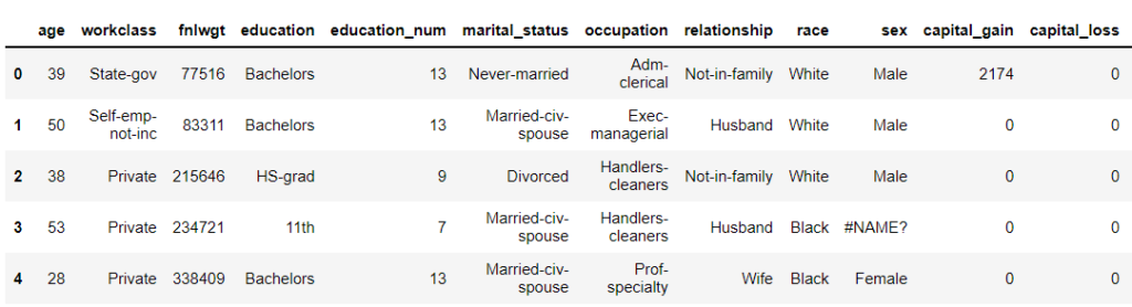
This data has NaN value as ‘#NAME?’. So setting na_values = [‘#NAME?’] will convert all [‘#NAME?’] values to NaN (Not a Number).
census = pd.read_csv("adult.csv",na_values = ['#NAME?'])
census.head()
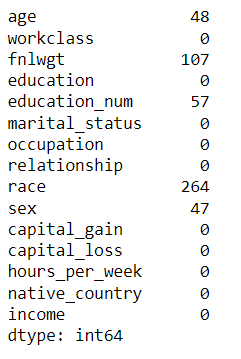
census.isna().sum()
What are the possible imputation techniques?
To impute NaN values, the pandas function fillna() can be used.
This imputation can be done with many appropriate strategies. In this article, we will look into major ways to get best results from the model.
1. Listwise Deletion or Complete Case: Drop Rows having NaN values:
When the NaN rows are very less when compared to the total data, for example, 20 rows when the entire dataset size is 10,000. Dropping 20 rows may not impact the model when the dataset is enough for prediction. However removing 20 rows for many column’s NaN values will definitely impact the model.
census = census.dropna(axis = 0,subset = ['sex','age'])
census.shape
(4905, 15)
census.isna().sum()
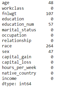
We have dropped the rows where age and sex columns are NaN. axis=0 specifies the rows.
After the removal, the data set turns to 4905. When removing rows for more features may end up reducing more data from the dataset.
2. Impute with mean/median/mode:
The another way is replacing NaN value with any appropriate substitutions.
- Impute NaN in Regression columns:
- When there are NaN values in numeric value columns, we can use either mean, trimmed mean, median or mode.
- Impute NaN in Categorical columns:
- Replace NaN with most frequent category of the feature. Using the function mode() will fill the NaN values with most frequent value.
- Replace with “Others” category.
- We can introduce another category as “Unknown“. If it already exists, then we can directly replace NaN with “Unknown”.
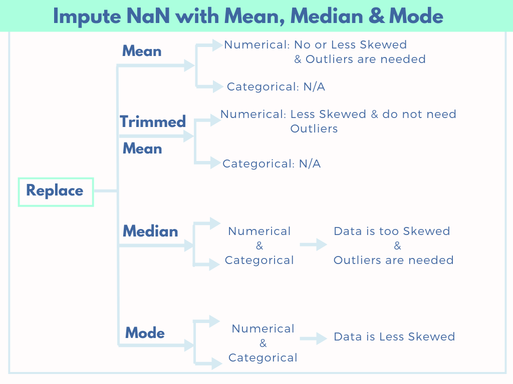
We will see when to use which statistical operation and how to do it.
When to use Mean for imputation?
The missing data can be filled with mean of the column’s values in the below cases.
Can be used only for numerical column.
Case #1: The data is roughly symmetric in Normal distribution or less skewed.
Case #2: Even thought the data is somewhat skewed with outliers and we need the outliers for the model. Example: Income – Outliers may exists but the income is too high in certain cases is also true.
Case #1: The data is normally distributed (symmetric) and the data is not skewed:
If the data is not normally distributed, then that means there are several data points are outliers. These outliers will make a great impact in mean values and the mean value will not represent the major data points.
For example, lets take the data points [5, 6, 3, 4, 5, 7, 100, 3, 8, 2].
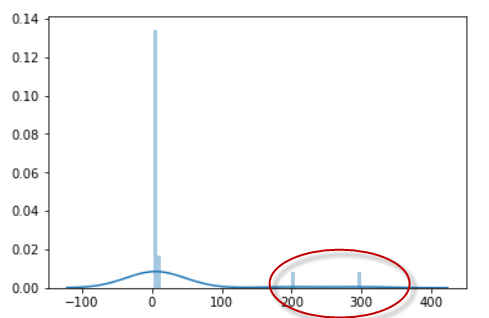
lst = [2, 3, 3, 4, 4, 4, 5, 5, 5, 6, 6, 6, 6, 7, 7, 7, 8, 8, 200, 300]

sns.distplot(lst)
The same list in distribution: the marked points are outliers.
from scipy import stats
import numpy as np

print("Mean:", np.mean(lst))
print("Median:", np.median(lst))
mode = stats.mode(lst)[0]
print("Mode:", mode[0])
Mean: 29.8
Median: 6.0
Mode: 6
Notice that the median and mode represents the data points but the mean value is not.
Lets check the normal distribution of the census data “hours_per_week” (hours_per_week) column.
#Exclude NaN
hours_per_week_selected_rows = census[~census['hours_per_week'].isnull()]
hours_per_week = hours_per_week_selected_rows['hours_per_week']

# Distribution plot
sns.distplot(hours_per_week)

print("Mean:", np.mean(hours_per_week))
print("Median:", np.median(hours_per_week))
mode = stats.mode(hours_per_week)[0]
print("Mode:", mode[0])
print("Minimum:",np.min(hours_per_week))
print("Maximum:",np.max(hours_per_week))
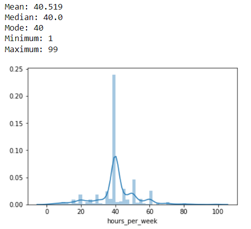
This distribution is symmetrically distributed. Thus the Mean, Median & Mode are same 40.
Also the Minimum & Maximum are not too far from the mean. 1 & 99.
census['hours_per_week'] = census['hours_per_week'].fillna(census['hours_per_week'].mean())
Case #2: Data is somewhat skewed with outliers and we need the outliers:
Thus we can use any one of the measures Mean or Median or Mode.
Lets check the another column “fnlwgt” (final weight).
#Exclude NaN
selected_rows = census[~census['fnlwgt'].isnull()]
fnlwgt = selected_rows['fnlwgt']

# Distribution plot
sns.distplot(fnlwgt)

print("Mean:   ", np.mean(fnlwgt))
print("Median: ", np.median(fnlwgt))
mode = stats.mode(fnlwgt)[0]
print("Mode:   ", mode[0])
print("Minimum:",np.min(fnlwgt))
print("Maximum:",np.max(fnlwgt))
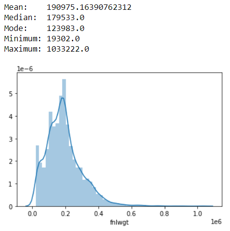
This distribution is somewhat/less skewed to the right side. Thus the maximum value is too far from the mean value.
However the mean value is just 1000 numbers greater than median.
In this case we have to check whether we need the outliers or not. If the outliers are needed, then we can use mean.
census['fnlwgt'] = census['fnlwgt'].fillna(census['fnlwgt'].mean())
When to use Trimmed Mean for imputation?
What is a trimmed mean?
The trimmed mean is the average of data after removing some large values (right skewed) and some very small values (left skewed).
How to find trimmed mean in python?
from scipy import stats

lst = [2, 3, 3, 4, 4, 4, 5, 5, 5, 6, 6, 6, 6, 7, 7, 7, 8, 8, 200, 300]

print("Mean:   ", np.mean(lst))
print("Trimmed Mean: ", stats.trim_mean(lst, 0.1))

print("Median: ", np.median(lst))
mode = stats.mode(lst)[0]
print("Mode:   ", mode[0])
Mean:    29.8
Trimmed Mean:  5.6875
Median:  6.0
Mode:    6
Here, stats.trim_mean(lst, 0.1) provides the trimmed mean after the 10% of outliers removed.
Can be used only for numerical column.
When distribution is somewhat skewed and the data has a few outliers and those outliers are not needed for the model. i.e. The outliers distort the analysis.
After removing the very large or very small data points, the skewness will be reduced. Thus the mean value will almost represent the data points.
Lets consider that we do not need outliers in the column final weight ‘fnlwgt’.
selected_rows = census[~census['fnlwgt'].isnull()]
fnlwgt = selected_rows['fnlwgt']

# Distribution plot
sns.distplot(fnlwgt)

print("Mean:   ", np.mean(fnlwgt))
print("Trimmed Mean: ", stats.trim_mean(fnlwgt, 0.2))

print("Median: ", np.median(fnlwgt))
mode = stats.mode(fnlwgt)[0]
print("Mode:   ", mode[0])

print("Minimum:",np.min(fnlwgt))
print("Maximum:",np.max(fnlwgt))
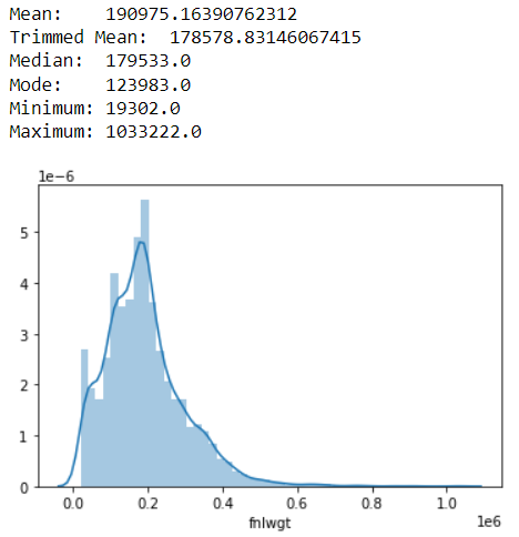
Notice that the trimmed mean after removing 20% of outliers is similar to Median. In this case, we can use Trimmed mean. In a case where we need outliers, using the median is similar to using the trimmed mean.
#Exclude NaN to find trimmed mean
selected_rows = census[~census['fnlwgt'].isnull()]
fnlwgt = selected_rows['fnlwgt']

trim_mean = stats.trim_mean(fnlwgt, 0.2)

print("NaN count before imputation:", census['fnlwgt'].isna().sum())
census['fnlwgt'] = census['fnlwgt'].fillna(trim_mean)
print("NaN count after imputation:", census['fnlwgt'].isna().sum())
NaN count before imputation: 107
NaN count after imputation: 0
When to use Median for imputation?
When the data is too skewed and we need outliers also in the data for analysis/model, then we can impute NaN with Median values.
print("NaN count before imputation:", census['fnlwgt'].isna().sum())

census['fnlwgt'] = census['fnlwgt'].fillna(census['hours_per_week'].median())

print("NaN count after imputation:", census['fnlwgt'].isna().sum())
NaN count before imputation: 107
NaN count after imputation: 0
When to use Mode for imputation?
Mode means that the most frequent value in the data.
Mode can be used for both numerical and categorical data.
For Numerical Data: When the data is skewed and a few values has high frequency, then mode will represent the best replacement for NaN.
For Categorical Data, the most frequent values/Mode is the best replacement for NaN.
census['race'] = census['race'].fillna(census['race'].mode()[0])
The race column is a categorical column.
census.race.value_counts()
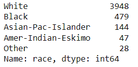
The white category is the most frequent value for race column. So we can replace NaN with White.
3. Impute NaN with ‘0’ or ‘Unknown’ or ‘Others’ values:
In some other data, replacing with mean value may not be suitable.
For example, while gathering data for fuel consumption, if a person is not owning any fuel using vehicle and using only a bicycle, then the petrol and diesel consumption will be 0. In this case we cannot replace that with mean/median values.
Similarly, in some other categorical values, using most frequent value may not be suitable. For example, in the census data, the categories for Race column are ‘White’, ‘Black’, ‘Asian-Pac-Islander’, ‘Amer-Indian-Eskimo’, ‘Other’ and NaN.
Here the others is used to mention very low frequent categories, i.e. 1 or 2 occurrences of some race categories. When comparing to the other race categories, consolidating the 1 or 2 counted categories as Others will not make any impact on performance of the model.
#Replace NaN with Others using fillna
census['race'] = census['race'].fillna('Other')

#Replace NaN with Others using replace function
census['race'] = census['race'].replace(np.nan, 'Other')

#Replace NaN with 0 - in case if we had NaN in capital_gain
census['capital_gain'] = census['capital_gain'].replace(np.nan, 0)
4. Impute NaN within group for a dependent variable
In the previous sections, we have imputed NaN using mean, trimmed mean, median or mode.
Suppose if we know that the corresponding variable depends on another variable, then directly replacing with any of the above statistical data will not makes sense.
For example, lets take the alcohol consumption data. If we are having the consumption rate variable and the age of the person. The age of the person is highly depends upon the consumption rate. For example, we know that 5 year old child and a new born baby will have 0 rate of consumption.
If you want to impute consumption rate for the entire entire data, then you are including both underage people like children and old people who crossed the age of 90 in the calculation. But for mean values these data points look like outliers for the data points having high consumption rate people.
When imputing a variable A which highly depends upon on another variable B, then imputations of variable A should be done with in the group of variable B.
For example, consider we are working on the below agriculture data.
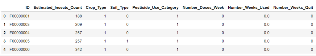
Now we have NaN values in Number_weeks_used column. This column indicates how many weeks the Particular pesticide category is used.
So, the column Number_Weeks_Used & Number_Doses_Week depends on the Pesticide_Use_Category column.
df_train.groupby('Pesticide_Use_Category').count()['Number_Weeks_Used']
Pesticide_Use_Category
1      740
2    57230
3    21888
Name: Number_Weeks_Used, dtype: int64
sns.barplot(x='Pesticide_Use_Category', y='Number_Weeks_Used' ,data = df_train[['Pesticide_Use_Category','Number_Weeks_Used']])
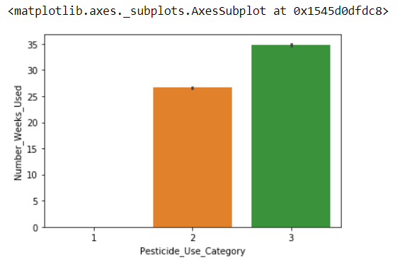
Impute Number_Weeks_Used within the group of Pesticide_Use_Category:
df_train['Number_Weeks_Used'] = df_train['Number_Weeks_Used'].fillna(df_train.groupby('Pesticide_Use_Category')['Number_Weeks_Used'].transform('mean'))
If a Categorical column needs imputation and it depends on another column, then we can use Mode() function.
df_train['Category_Column'] = df_train['Category_Column'].fillna(df_train.groupby('Dependent_Column')['Number_Weeks_Used'].transform('mode'))
Impute regression column within a group using mean/Trimmed Mean/Median.
Impute categorical column within a group using the mode.
5. Drop columns if >60% of data is missing
When most of the data points are NaN in a column, we cannot predict anything with that feature.
So if a feature has only less values, we need to do any one of the following:
Try to collect proper data for that feature again
Remove that feature from data and work on the remaining data.
census.drop(['race', 'capital_gain'], axis=1, inplace=True)

#OR

census = census.drop(['race', 'capital_gain'], axis=1)

#OR

census = census.drop(columns=['race', 'capital_gain'])
Conclusion:
In this post we have seen 4 major ways to impute NaN values.
This is a Part II of 5 part series of Data Pre-Processing tutorial.