In any Machine Learning or Deep Learning Models, our common goal is to reduce the cost function.
A famous and well known technique to reduce the Cost Function is Gradient Descent.
In Machine Learning, we use Gradient Descent to optimize the Co-efficients of the Linear or Logistic function. To learn how Gradient Descent works, please check this article.
In Deep Learning, we use Gradient Descent to optimize the weights of the connections between neurons, which is finally the coefficients.
Many variants of SGD are proposed and used nowadays. However all the optimizers has their own shortcomings. We can choose the optimizer based on the issue and usage.
One of the most popular ones are Adam (Adaptive Moment Estimation)
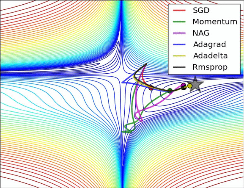
The below animation is an excellent illustration of comparison of optimizers made by Alec Radford. Unfortunately the Adam optimizer is not mentioned in this illustration.
Standard Optimizers:
When discussing about Optimization, the first word comes to our mind is Gradient Descent.
There are 3 variations of Gradient Descents. Each type has its own advantages and disadvantages.
Batch Gradient Descent
The Vanilla version of Gradient Descent is Batch Gradient Descent.
In this technique, we take the entire data set and computes the Gradient Descent.
i.e. For each epochs, the entire dataset is used in the calculation of MSE.
The Disadvantage of this as we are taking the entire data set, obviously it increases the complexity.
And so it is very slow as for a Neural Network.
Stochastic Gradient Descent
In the previous technique, the cause of the disadvantage is taking the entire dataset into the computaion.
With SGD, we overcome it by taking 1 random sample from the entire dataset.
This makes the computation simple.
But the problem is, even though it definitely converges to the optima, the gradient descent will jump widely (oscilate more) which takes more iteration.
In some iterations, we may take the noise in account.
So there wil be a high variation in weights.
Mini batch Gradient Descent
This type is a hybrid of first 2 variations.
In this type, we take a random set of sample and compute the Gradient Descent.
As we take a set of random sample instead of 1 the noise and variance will be reduced which helps to have the steady convergance.
Adaptive Optimization Algorithms:
In addition to the above Gradient Descent Algorithms there are some Adaptive Optimization Algorithms which works along with any of the above GD algorithms.
These algorithms are gaining popularity as it makes the convergance quick and smooth.
- Momentum
- Nesterov accelerated gradient(NAG) (aka Nesterov Momentum)
- Adagrad — Adaptive Gradient Algorithm
- Adadelta
- RMSProp
- Adam — Adaptive Moment Estimation
- Nadam- Nesterov-accelerated Adaptive Moment Estimation
from keras import optimizersMomentum:
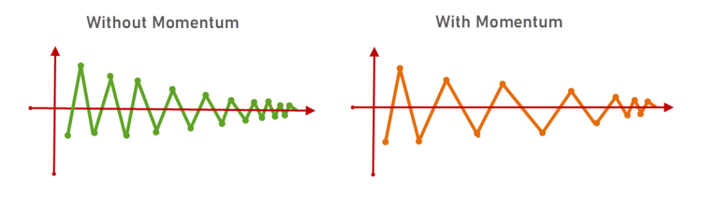
Momentum is a variation of Standard Gradient Descent which considers the past gradients to smooth out the update. It calculates an average of the past gradients, and then use that gradient to update weights instead.
So the oscillation gets reduced.
It works faster than the standard gradient descent algorithm.
vt = γvt−1 + η∇θJ(θ) (1)
θ = θ − vt (2)
γ is the update vector of the past step to the current update venctor.
momentum = optimizers.SGD(learning_rate=0.01,
    momentum=0.8,
    nesterov=False,
    name='SGD-Momentum')
model.compile(optimizer = momentum, loss = 'categorical_crossentropy', metrics = ['accuracy'])
Nesterov accelerated gradient(NAG) (aka Nesterov Momentum):
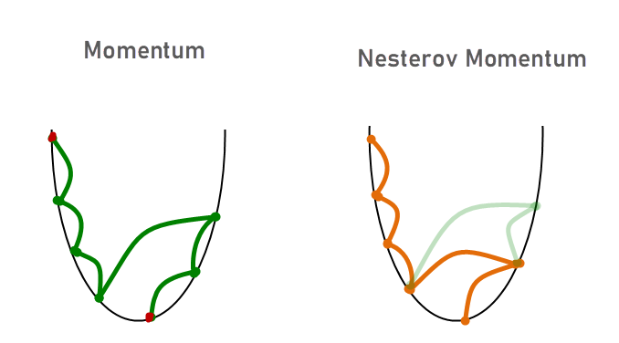
Well, Momentum was smart enough to look back and take steps.
But What if we know about the forward step too? That’s exactly what NAG does.
vt = γ vt−1 + η∇θJ(θ − γvt−1) (3)
θ = θ − vt (4)
(θ − γvt−1) is the approximate value that describes the next point.
nesterov = optimizers.SGD(learning_rate=0.01,
    momentum=0.8,
    nesterov=True,
    name='SGD-Momentum')
model.compile(optimizer = nesterov, loss = 'categorical_crossentropy', metrics = ['accuracy'])
Adaptive Gradient – Adagrad:
Earlier in all algorithms we were not changing learning rates.
Adaptive Gradient algorithm works in a way that learning rates will be changing w.r.t the number of iterations.
In the previous optimization techniques, the value of η will remain constant for all the iterations.
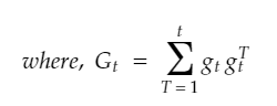
But in Adagrad, we will divide the η value by the sum of the outer product of the gradients until time-step t. We mention this term as Gt.
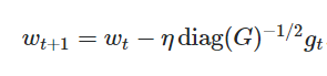
By dividing η this value directly will give worst result.
“diag” -> Gt is multiplied with a diagonal matrix so that the value will not vanish (will not become zero).
As we are dividing the learning rate by sum of past iterations, when the iterations increases, the learning rates will be decreased.
Disadvantage:
The only problem with this algorithm is, as the learning rate decreases, the convergence becomes slow.
Thanks to: https://medium.com/konvergen/an-introduction-to-adagrad-f130ae871827
Adadelta:
Adadelta is an extension of Adagrad. This algorithm addresses the disadvantage of Adagrad. It controls the shrinking learning rate when iterations increases.
Adagrad computes the learning rates based on all the past gradients. But in Adadelta, it only takes the recent gradients in account.
For more information please check the original Adadelta paper.
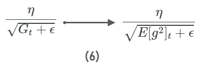
RMSprop (Root Mean Square Propogation) :
This optimizer tries to overcome the shrinking learning rate by using the average of squared gradients.
With this optimizer, the learning rates will be adjusted automatically.
rmsp = RMSprop(lr=0.00025, epsilon=0.01)
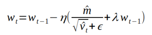
model.compile(optimizer = rmsp, loss = 'categorical_crossentropy', metrics = ['accuracy'])Adam (Adaptive Moment Estimation) :
Adam optimizer is a hybrid of RMSProp & Momentum.
adam = optimizers.Adam(learning_rate=0.01,
    beta_1=0.9,
    beta_2=0.999,
    epsilon=1e-07,
    amsgrad=False,
    name='Adam')
model.compile(optimizer = adam, loss = 'categorical_crossentropy', metrics = ['accuracy'])
Thanks to:
https://medium.com/@nishantnikhil/adam-optimizer-notes-ddac4fd7218
https://ruder.io/optimizing-gradient-descent/index.html#rmsprop