
In this article we will explore why we need Logistic, how can we derive Logistic Regression from Linear Regression and a few more important facts in mathematics.
Let’s Recall the nature of Linear Regression:
In Linear Regression, we try to estimate the continuous variable Y depending on any type of variable X when there is a linear relationship between X & Y.
If we say linear relationship, it means, there is a pattern between X & Y. For an amount of increase in X, we identify a constant change in Y.
This is mentioned as a line equation. Y = mX + c
Let’s consider c as 0 for now to understand better.
Then the equation becomes Y = mX.
If m =2, => Y = 2X. i.e. for 1 unit of rise (Y), there is a 2 units of run (X).
So, in Linear Regression, the change of Y is constant for any value of X.

Take a line with coordinates (1,2), (2,4) & (3,6)…. You can see that (Graph #1) the Y value constantly increase 2 times that of X.
For 1 unit of run (x), there is a 2 unit of raise (y).

Why we need Logistic Regression?
In this graph (Graph #2) also there is a constant change in Y for any value of X.
So that means there is a ratio between X & Y values.
Consider that Y value is not continuous. If the Y value is discrete, then it is bound to the mentioned discrete values.
If the problem is binomial, then Y value can only be 0 or 1.
For example, Success or Failure, Yes or No, Survived or Not Survived.
In this case all our Y values will be either 0 or 1. Neither in-between nor beyond. Then applying the linear regression becomes like this.
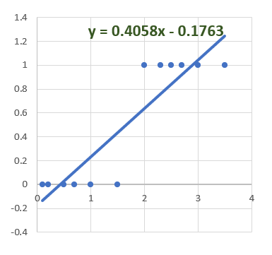
But the real problem occurs when we predict values.
In the above graph, it says Y value is equal to 0.4058x — 0.1763.
For a higher value of X, the Y values goes beyond 1. But we need either 0 or 1.
Then how can we map/normalize the values of Y within 0 & 1 for any corresponding values of X.
We need a constant effect in Y for a value of X, but it should not go beyond 1 or below 0.
We need to somehow map/transform the Discrete Y values with the continuous Y values that has a constant effect with respect to X.
Now let’s see what we have in the world of mathematics for this issue!
Transformation of Linear to Logistic Regression:
We have Linear regression algorithm that works well for continuous values.
But when the Y values are discrete, we cannot map it with Line equation’s Y value.
We need to map these probability discrete values with continuous value for which we can use Linear Regression Algorithm.
In other words, we need to transform the Linear Regression algorithm which can predict a continuous value that ranges from -infinity to +infinity to predict discrete value.
Now let’s see what we have in the world of mathematics for this issue.
Logistic regression can be binomial, ordinal or multinomial.
Binomial or binary logistic regression — two possible outcomes “0” and “1” Example: Success/Failure, Yes/No.
Multinomial logistic regression — More than 2 outcome which cannot be ordered. Example: Course selection: Course A/ Course B/ Course C.
Ordinal logistic regression — Similar to multinomial but the outcomes can be ordered. Example: Movie Ranking: Excellent/ Good/ Average/ Bad.
Lets take Binomial/ Binary Logistic Regression in our discussion. When there are two possible outcomes, it could be compared to the Bernoulli’s Distribution.
The Bernoulli distribution is a probability distribution of a random variable using either 0 or 1. As this uses only 2 classes, it is a binary/binomial model.
The Bernoulli distribution, named after the Swiss mathematician Jacques Bernoulli (1654– 1705), describes a probabilistic experiment where a trial has two possible outcomes, a success or a failure.

If all the possible outcomes are 100 %, if the probability of success is 60% then all other remaining chances automatically goes to failure. So 100–60 = 40%.
If the success is considered as 1 and failure as 0, the total chance is 0+1 = 1.
Let’s generalize it to look more in mathematical way, If the probability of success is p, then the probability of failure is the remaining all other chances.
So, probability of failure can be written as 1-p, if we want to denote it with different variable, you can say that as q = 1-p.
However, having it as 1-p makes easy to understand when it comes to derivations.
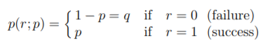
Here r is the result.
The above distribution is generalized to the below form:
P(x) = p^x * (1-p)^(1-x)
To understand the above equation, let’s plugin 0 & 1 as x in this equation.
For x= 1 (success), p(1) = p¹ * (1-p)^(1–1) = p * (1-p)⁰ = p * 1 = p
For x= 0 (Failure), p(0) = p⁰ * (1-p)^(1–0) = 1* (1-p)¹ = 1-p
Now you get the success and failure values of p(r; p) equation.
Probability is the number of times success occurred compared to the total number of trials.
Let’s say out of 10 events, the number of times of success is 8, then
Probability of Success = 8/10 = 0.8
Probability of Failure = 1- 0.8 = 0.2
Now we found what our Y value’s nature is. It is a binomial value and it can be described as probability of success and failure.
Odds Ratio is another measurement to know how likely it is that something will occur.
Odds are the number of times success occurred compared to the number of times failure occurred.
i.e. Odds are defined as the ratio of the probability of success and the probability of failure.
=> Probability of success : Probability of failure
which can be denoted as,
Odds Ratio (Success) = Probability of success / Probability of failure
Odds Ratio (Failure) = Probability of failure / Probability of success
We can determine Odds ratio from Probabilities.
If the probability of Success is p,
Odds ratio = p/(1-p)
Odds ratio ranges from 0 to infinity.
If the probability of success is 0.8, then odds ratio is
OR = 0.8/(1–0.8) = 0.8/0.2 = 4
=> 4/1, That is Odds ratio is 4:1.
For each 4 successes there is 1 failure.
If the p value is 0.25, the OR = 0.25/0.75 = 1/3
Then for each 1 success there are 3 failures.
Finally, we found a pattern.
But this odds ratio starts from 0 as probability starts from 0 but ranges up to infinity.
No worries! we have a Logarithm to change its range.
Let’s see what are the properties of logarithm.
log(x) is a base 10 logarithm. Can also be written as log10(x).
ln(x) means the base e logarithm. Can also be written as loge(x).
Log and Exponential are inverse to each other. e^x is the inverse of ln(x).
Loge(a) = e^x


You can clearly see that Exponential is the inverse of log.
Log of any values can range from -infinity to +infinity.
Below table illustrates the transformation we made so far:
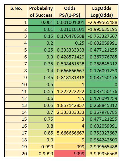
You can see that for the given values Log odds ranges from -2 to 3. For different values of p, it can range from -infinity to +infinity.
So, we have transformed the probability value as log odds. This transformation is called Link Function.
Transform Linear to Logistic:
In the Linear Regression algorithm, our Line equation is Y = mX + c
You can use any fancy notations for X slope m and y intercept c.
Experts write it as y=β0+β1x1
Explanation from Minitab:
A link function transforms the probabilities of the levels of a categorical response variable to a continuous scale that is unbounded. Once the transformation is complete, the relationship between the predictors and the response can be modeled with linear regression.
For example, a binary response variable can have two unique values. Conversion of these values to probabilities makes the response variable range from 0 to 1.
When you apply an appropriate link function to the probabilities, the numbers that result will range from −∞ to +∞.

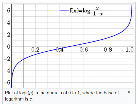
You can see that it is a S shaped curve.
The inverse of this function brings us the Sigmoid curve.
The inverse-logit function is called as the Logistic Function.
(To know more about inverse function, watch this video. It is explained very well using simple examples.)
Key points from Wiki:
The logit in logistic regression is a special case of a link function in a generalized linear model: it is the canonical link function for the Bernoulli distribution.
The inverse-logit function (i.e., the logistic function) is also sometimes referred to as the expit function.
If p is a probability, then p/(1 − p) is the corresponding odds; the logit of the probability is the logarithm of the odds, i.e.

The “logistic” function of any number ∝ is given by the inverse-logit:

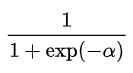
The above function is the Sigmoid function.
We have reached the logistic curve that fits very well for our binomial data.
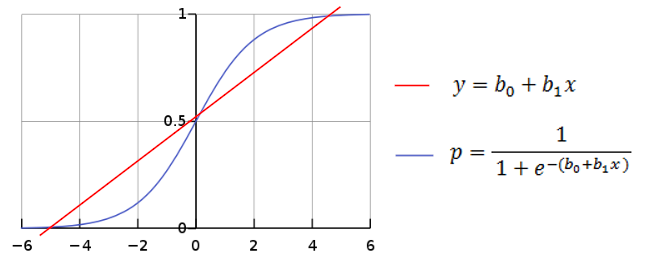
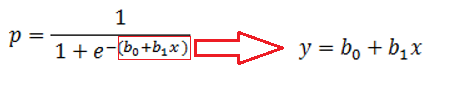
From the equations of line and sigmoid function you can see that if we know the x coefficients and slopes, we can convert it to the required probability values.
The Sigmoid function is a mathematical function having S shaped curve which ranges between 0 & 1.
This function converts a value x into a probability of an event.
If the probability value, i.e. the outcome of the sigmoid function value p >= 0.5, then the output is marked as 1 (true/positive/success).
If p < 0.5, then it is marked as 0 (false/negative/failure).
Thus for any value of x, we have a constant effect in y and it could be ranged between 0 & 1 and also it could be classified to a discrete value.
Conclusion:
In this article, we have seen the Probability, Log odds and finally we transformed the known Linear Regression to unknown Logistic Regression.
Logistic Regression works similar to Linear Regression first to find the X coefficients and slope, in addition to that it applies the Y predicted value into the sigmoid function to map the received real value (ranges from -infinity to +infinity) into a binary value (ranges from 0 to 1).
🤞Hope you can understand the concept of Logistic Regression now.
This article is more mathematical, but implementing a model in Python is as easy as we did in Linear Regression. It is just a line of Python code.
Lets explore the Cost function in Logistic Regression Part II— Cost Function & Error Metrics and & programming section in a new post.
If you find any corrections, I am really grateful to know that, please add it in comments.
Thank you! 👍
Thanks to:
Like to support? Please just click the heart icon ❤️.
Happy Programming!🎈