Ever thought about doing magic or predict future? Here is the guide! lol! In this article lets go programming with sklearn package to explore Linear Regression and learn how to do prediction with Linear Regression.
We have seen enough theories about Linear Regression in previous posts of this series. If you want to have a glance, below are the details.
- Linear Regression — Part I
- Linear Regression — Part II — Gradient Descent
- Linear Regression — Part III — R Squared
Reading Data:
Import necessary libraries to read the data.
import pandas as pd
I have downloaded the data from Kaggle. Thanks to Kaggle, they are giving lots of data for beginners to try and learn. Link to Kaggle to get data for Linear Regression.
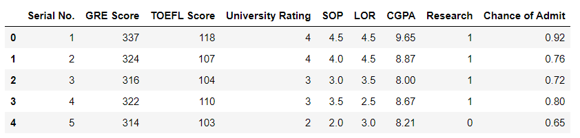
I have taken a Admission Prediction data set. Lets explore the data:
df = pd.read_csv("Admission_Predict_Ver1_1.csv")
df.head()
Data Pre-Processing:
Our next step is Pre-Processing the data to get more accurate results.
df.isnull().sum()
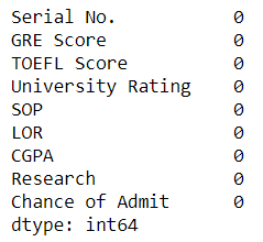
But luckily as it is a data set mainly given to beginners, it has no null values and data is also clean. All the values are continuous values and not categorical values.
We will see how to use categorical values later in a new post.
Lets check the correlation between Independent & Dependent values.
df.corr()
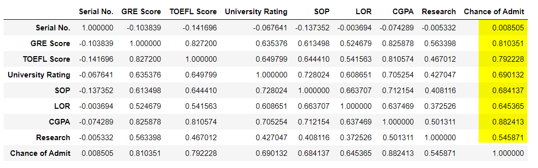
df.columnsIndex(['Serial No.', 'GRE Score', 'TOEFL Score', 'University Rating', 'SOP', 'LOR ', 'CGPA', 'Research', 'Chance of Admit '], dtype='object')
Out of all the columns, S.No is not related to the Chance of Admit. So we can remove it. And the value that is going to be predicted is ‘Chance of Admit’. Having this column in X does not make sense as change in this column will be exact equal to the change in Y which is the same column for which we are going to predict values.
If you still want to know, then just give it a try , you will end up with 100% accuracy. i.e r² value will be 1. That’s happy to see but not useful anymore.
Be happy for a minute and lets comeback to the reality!
In future if you get 100% accuracy immediately, first check whether you added Y in X! lol! I have done that enough # of times to remember this!
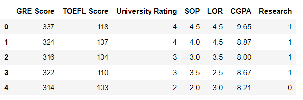
Here I have removed ‘Serial. No’ & ‘Chance of Admit’ from X and have only ‘Chance of Admit’ in Y.
X = df.drop(['Serial No.','Chance of Admit '],axis = 1)
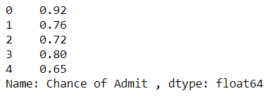
y = df['Chance of Admit ']
Split the entire data frame into X & Y parameters. Basically the X parameters are the Independent Variables and Y parameter is the Dependent Variable that we need to predict. Lets look at the X & Y variables.
X.head()
y.head()
Test Train Split:
Now we need to split the data into train & test sets. We train our model with train set and verify the model with test set.
Usually the train set should be higher than test set so that we get more data to for learning. Also the accuracy will be different for different split.
Example splits are 60–40, 80–20 or even 73–27.
You can just mention the test size so that the train set will be automatically the remaining. But how to select which rows for test?
This split should be done randomly.
sklearn has package train_test_split which allows us to split the data into train and test in a random manner. You can also control the randomness using the parameter random_state.
If you and I use same int value for this parameter then we both will have a same set of test & train data for the same data set.
test_size parameter takes value <= 1 i.e. 0.33, 0.4 to mention the percentage of data for test set.
Import necessary packages. I will explain one by one when it is required.
from sklearn.model_selection import train_test_split
from sklearn.linear_model import LinearRegression
from sklearn.metrics import r2_score

X_train, X_test, y_train, y_test = train_test_split(X, y, test_size=0.4, random_state=101)
Lets see how many rows train & test data set has:
X_train.shape
Output: (300, 7)
X_test.shape
Output: (200, 7)
Creating Linear Regression Model:
Now we are done playing with data. Lets get into the real game! Lets create a Linear Regression model to predict the Chance of Admit of a new student.
sklearn provides a lots of packages for various algorithms. Here we are using LinearRegression() which creates a new object for this algorithm. with this object, we can fit our data and use this object to get the parameters of our model.
lr = LinearRegression()  #Object Created
lr.fit(X_train, y_train) #Data given into the LinearReg. object
Done! Congratulations, you have created your first model.
Yes! Simple isn’t it? Lets see what we can get from this model!
lr.coef_
Output:
array([0.00145221, 0.00302388, 0.00809642, 0.00672185, 0.01318406,
0.12002891, 0.02477235])- These are the Coefficients (slopes) of the X Variables — GRE Score, TOEFL Score, University Rating, SOP, LOR, CGPA, Research.
- So 0.00174541 GRE + 0.00280216 TOEFL + 0.00675831 University + 0.0061299 SOP + 0.01492133 LOR + 0.11902878 CGPA + 0.01943883 * Research
lr.intercept_
Output:
-1.200250569689947This value is the Y Intercept. So our Y line equation becomes,
ChanceOfAdmit = -1.2567425309612157 + 0.00174541 GRE + 0.00280216 TOEFL + 0.00675831 University + 0.0061299 SOP + 0.01492133 LOR + 0.11902878 CGPA + 0.01943883 * Research
What next? Lets test our model.
Using the predict method of the lr object, by sending in the x_test values, we can predict the y_test values. As we already have the original y_test values, we can now validate our model.
predicted = lr.predict(X_test)
r2_score(y_test, predicted)
Output:
0.8251757711467193We have predicted Y values for test set and compared it with the true values using the r1_score function from the package sklearn.metrics. Our model’s accuracy is 0.8251757711467193. That means our predictions will be 82% correct.
- Lets check!
y_test.head(10)
Output:
18     0.63
361    0.93
104    0.74
4      0.65
156    0.70
350    0.74
32     0.91
205    0.57
81     0.96
414    0.72
Name: Chance of Admit , dtype: float64
Get predictions for first 10 rows.
print(predicted[0:10])
Output:
[0.74116361 0.91082451 0.81024774 0.62183042 0.64643854 0.69311918
 0.91233928 0.51828756 0.95333009 0.73419915]
Here we have predicted for the test data we had.
Now you can see that most of our predictions are very close.
Lets predict for new data.
new_y = lr.predict([[347, 120, 4.5, 4.7, 4.7, 9.8, 1]])
print(new_y)
Output:
[0.99758071]Another test:
new_y = lr.predict([[250, 90, 2, 2.5, 4.7, 7, 1]])
print(new_y)
Output:
[0.39488945]Now you have got your model and you can predict Chance of admission for any scores.
We are done training and testing the Linear Regression model and predicted for chance of admission as well.
Conclusion:
In this article we have learned how to do Linear Regression model and how to predict values.
I will come up with more research and some more interesting facts in Machine Learning and see you in my next post!
Special thanks to Kaggle for datasets!
Please explore this algorithm with various data and try it in python. Dont forget to drop your ideas in comments. It will be useful for me and all the readers!
Thank you!
Like to support? Just click the heart icon ❤️.
Happy Programming!