Linear Regression is a linear approach to model the relationship between a two or more variables by fitting a straight line i.e. linear, to predict the output for the given input data.
To perform Linear Regression, Data should accomplish the below constraints:
- Data should be Continuous.
- There should be a Correlation & Causation exists between Independent & Dependent Variable.
To research deeper into the concept of why Regression made on Continuous and Correlated data, please check this page.
If the Linear Regression is made on one independent variable, plotting of data will be similar to the below scatter plot.
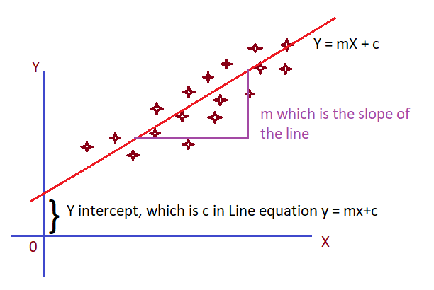
X — Independent Variable i.e. Input training data
Y — Dependent Variable, i.e. Output data
In mathematical way, every line has an equation. Y = mX + c
For a straight line the m & c value will be constant and X is a set of values.
slope = m = rise/run = dy/dx i.e. Change in Y/Change in X
For example, if (m, c) is (2,1) then the equation becomes Y = 2X + 1
Line of best fit:
In the above example linear regression model, as the data is in a good correlation, a line can be drawn such that it runs in a way that all the points in the graph is most possibly near to the line, which is called a line of best fit. Thus, we can be sure that for any new value of X, the Y value is where the perpendicular line from X point meets the Straight line.
Let ŷi is the Y value as predicted by the line of regression when x = xi.
Then for each point there is an error/difference between the predicted and actual value which can be defined as Ei = yi — ŷi.
As an overall error, we need to find this difference for all the existing input data and sum its square (SSE)which we will see in this article (Section Cost Function).
Now the question is for what value of m & c, this SSE value will be most possible minimum?
To find this m & c value of a Linear Regression model there are many methods available.
But the most known methods are,
- Ordinary Least Squared. — Non-Iterative method. Find m & c from the given data using formulas.
- Gradient Descent. — Randomly take m $ c and reduce the error alliteratively.
- Maximum Likelihood Estimation.
In this article, we will be learning about Ordinary Least Squared method to find the best fit line.
As Gradient Descent needs more clear understanding, I will be posting it as a separate article.
Least Squared method:
To find the best fit line for our data, Least Squared method is a mathematical way for find the slope and y intercept.
i.e. We need to find a mapping function/pattern in which Y values are changing depending up on the X values. For linear regression it is a straight line.
The mapping function is Y = mX + c.
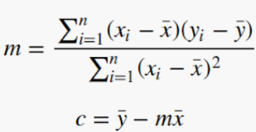
To find m — slope & c — intercept,
It is easy to understand this concept if we do it in MS. Excel.
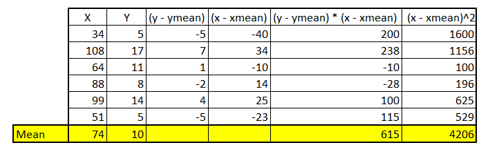
In the above table we have found the numerator and denominator of the slope formula.
Let’s find the slope,
Slope m = 615/4206 = 0.146
Now we can find C by the above-mentioned formula.
C = 10 — (0.146 * 74) =-0.818
So, a line that runs with the slope of 0.146 & y intercept of -0.818 is the best fit line for our data.
Cost function:
Even though the found line is a best fit line, not all the point may lie in the best fit line. Isn’t it?
Then how can we call this difference/error?
How to know what is the measure of the error for the best fit line?
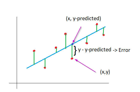
In the above graph u can see that the distance between y & y-predicted as error.
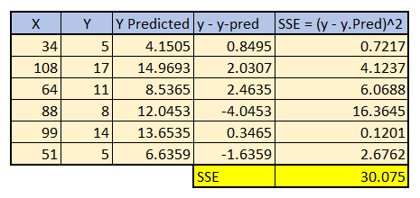
When we collect all the errors and sum its squares, that value becomes cost function of this best fit line.
As this is the line with slope of 0.146 & y intercept of -0.818 is the best fit line, this calculated cost is the most minimum for this example.
In terms of mathematics, the formula for Cost Function is,
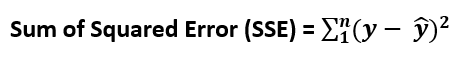
For the above given example, the SSE is 30.075.
Conclusion:
We have learned how to do linear regression using Ordinary Least Squared method and what is the cost function.
Congratulation to you on taking the first step in machine learning.
Please continue reading Linear Regression — Part II — Gradient Descent to know about Gradient Descent method to minimize SSE.
Until then Bye & Happy Programming.