Linear Regression — Part II — Gradient Descent

Gradient descent is an optimization algorithm used to minimize a cost function (i.e. Error) parameterized by a model.

We know that Gradient means the slope of a surface or a line. This algorithm involves calculations with slope.

To understand about Gradient Descent, we must know what is a cost function.

Cost function(J) of Linear Regression is the Root Mean Squared Error (RMSE) between predicted y value (predicted) and true y value (y).

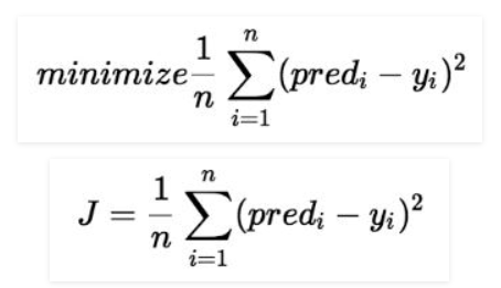
For a Linear Regression model, our ultimate goal is to get the minimum value of a Cost Function.

To become familiar about Linear Regression, please go through Linear Regression — Part I.

First Let us visualize how the Gradient Descent looks like to understand better.

As Gradient Descent is an iterative algorithm, we will be fitting various lines to find the best fit line iteratively.

Each time we get an error value (SSE).

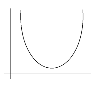
If we fit all the error values in a graph, it will become a parabola.

What is the Relationship between Slope, Intercept and SSE? Why Gradient Descent is a Parabola?

To answer these 2 questions, Let’s see the below example.

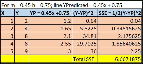
You can notice that I took random value of m = 0.45 & c = 0.75.

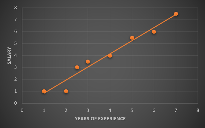
For this slope and intercept we have come up with a new Y predicted values for a regression line.

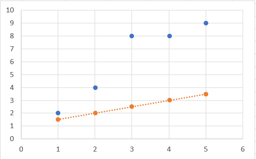
In the above graph, blue color dots are Original Y values & Orange color dots are Y predicted values that we just found with m = 0.45 & c = 0.75. We can clearly say that this line is not a best fit line for this data.

The total SSE for this iteration is 6.66 approximately.

Then let’s do the iterations by decreasing the m & c values randomly and the results are given below:

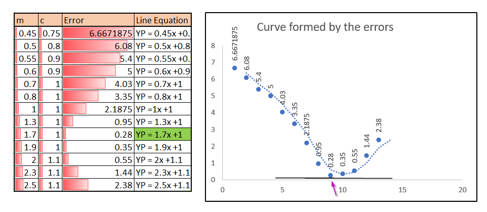
In the above table, we can see that for different values of m & c the error value decreases gradually and from a point it starts increasing again.

If we plot a graph for all the error values alone then that will look like a curve as shown in the right side.

Now we are going to plot all the lines that formed with above m & c values in our original graph (Column: Line Equation):

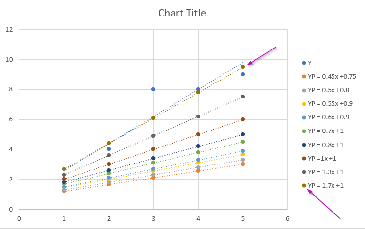
You can see that the pink marked line is formed with m as 1.7 & c as 1 which produces the minimum error of all other m & c values in the m, c & Error table. The blue color line is the best fit line produced by excel itself. Our line YP = 1.7x +1 is closest to the best fit line.

If we go into the iterations seriously with minimum change in m/c values, we will be hitting the best fit line.

In the parabola graph, we can identify that the error 0.28 is the minimum and it was produced by the line equation YP = 1.7x +1.

More than 1 Independent Variables:

Where there are only one Independent Variable X, the Linear Regression graph will be 2-Dimensional and the best fit will be a line.

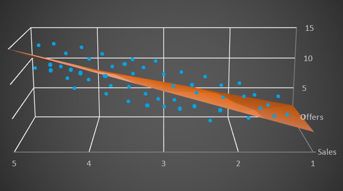
When there are 2 independent variables, the 2-D area becomes a surface/space of 3 Dimensional and the best fit become a Plane.

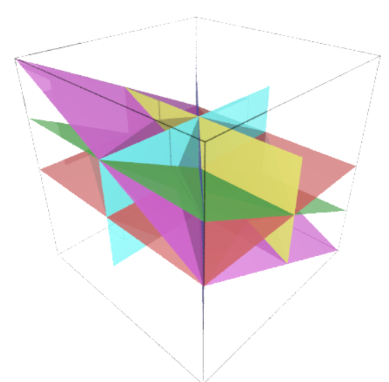
When n variables (n>2) exists, then the n-Dimension area becomes a n-Dimensional space and the best fit becomes a Hyperplane. Practically it is more complex to plot the n dimensional graph.

When Linear Regression is in 2-Dimensional, the Gradient Descent Error Graph will be formed as a Parabola.

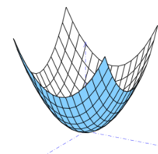
When the Linear Regression is in 3 Dimensional, the Gradient Descent will become elliptic paraboloid.

How to find the minimum cost?

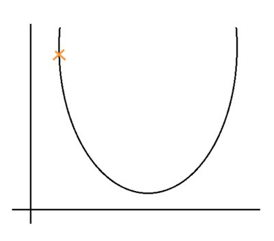
We found that all the possible error values form a parabola (or paraboloid in 3D) and the most minimum lies in the deepest of the curve.

Step #1: Take a random value for m & c. For any random values of m & c, the error value will not necessarily to be minimum. Let’s say it is somewhere in the parabola.

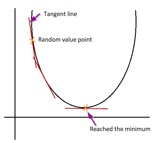
Step #2: Now we need to find, in which direction the slope is reducing so that we can reach the deep of the parabola.

This is when partial derivatives come to play.

We can compare descending from top of a para bola/paraboloid, we have to reduce the slope of the curve to reach its bottom.

Let me explain clearly. If you draw a tangent line in the point which u took as a random value, it is the slope of the curve in that point. Reducing the slope of the line will move down in the curve.

In which rate we have reduce the value is reducing the slope of the line.

Basically, to reduce the slope, we can use Partial Derivative in first order to get the reduced slope. Below is the update rule for m & c using partial derivative.

Update Rule:

Step #3: We need to change the m & c values using the update rule and know the new SSE value. Iterate this process until we reach the global minimum.

Things to remember:

1. m & c should be updated simultaneously. We should not update m fist then apply the value of new m to update c.

2. Learning rate is usually 0.01 but not necessarily to be 0.01 for all models. Highest learning rate will reduce the m & c values rapidly and it may skip the global minimum (a fancy word to mention the deepest point in parabola) value.

3. Even for a fixed value of learning rate, once you are near to the global minimum, your steps will be automatically smaller. You do not need to reduce the learning rate often.

Conclusion:

1. Gradient Descent is an iterative method, unlike Least Squared method, we will be taking a random value for slope m & intercept c of a best fit line.
2. The resultant SSE value (J or Cost) value may not be the minimum.
3. Identify the direction of most negative slope and step in to that direction. This is where partial derivatives enter the play.
4. Then we will do this iteratively with a learning rate until we get the minimum of all errors.
5. For the final minimum SSE, the used m & c value are the final outcome. The line set with final m & c is the best fit line.

Okay! We reached the end of our article.

Yes! I can hear you saying “Hey! how can you reach the end without a program”.

In the next part of this article, we will be looking at the error metrics (Linear Regression — Part III — R Squared) and then we will be going programmatically in python.

Until then Bye & Happy Programming!

Thanks to:

Coursera: https://www.coursera.org/learn/machine-learning/home/welcome