
Hello Everyone!!! Its an immense pleasure to write today as this is the first post I am able to write in 2021. Happy New Year!!! 🥳 🎂 🎉 In this article we are going to see the continuation of Deep Learning techniques. We are going to see an Deep Learning model with a Classification Example.
In our last article, we learned to use a simple Neural Network to solve regression problems – Artificial Neural Network Explained with an Regression Example.
If you missed the prequels, please check below:
Artificial Intelligence – A brief Introduction and history of Deep Learning
How Neurons work? and How Artificial Neuron mimics neurons of human brain?
Artificial Neural Network Explained with an Regression Example
Classification Example Dataset:
For easy use and easy to download, the breast cancer dataset from sklearn.datasets has been taken.
from sklearn.datasets import load_breast_cancer
from sklearn.model_selection import train_test_split

whole_data = load_breast_cancer()

X_data = whole_data.data
y_data = whole_data.target

X_train, X_test, y_train, y_test = train_test_split(X_data, y_data, test_size = 0.3, random_state = 7)
Finally we have the data set of 398 records for training and 171 records for testing with 30 features. Even though this is a very less data for deep learning, we are using this for experimental purpose.
Documentation of dataset: http://scikit-learn.org/stable/modules/generated/sklearn.datasets.load_breast_cancer.html#sklearn.datasets.load_breast_cancer
X_train.shape, X_test.shape, y_train.shape, y_test.shape

Output:
((398, 30), (171, 30), (398,), (171,))
Model Creation:
from keras.models import Sequential

model = Sequential()
A sequential model is created. Lets add deep learning layers to it.
# Keras model with two hidden layer with 10 neurons each
model.add(Dense(10, input_shape = (30,)))
# Input layer
model.add(Activation('sigmoid'))
model.add(Dense(10))
# Hidden layer
model.add(Activation('sigmoid'))
model.add(Dense(10))
# Hidden layer
model.add(Activation('sigmoid'))
model.add(Dense(1))
# Output layer => output dimension = 1 since it is regression problem
model.add(Activation('sigmoid'))
Here it can be noticed the input layer is having input shape of 30. And also 10 is mentioned in first line itself.
Now most of us may have a question, which is the exact input shape? 30 or 10?
The first layer that gets input is the input layer which is having 30 neurons here. each 1 input node is for each feature. the next layer is the first hidden layer which is having 10 neurons.
Also we can see that the output layer is having only 1 neuron. Why it is not having 2 neurons as the target variable is a binary class (1- malign, 0 – benign)?
This one neuron output value will be the probability value between 0 and 1 as we are using sigmoid activation in output layer. The probability value can be determined as 0 or 1n based on the threshold of 0.5.

Now we have constructed the neural network. Lets compile it with optimizers and loss function.
from keras import optimizers

sgd = optimizers.SGD(lr = 0.01)    # stochastic gradient descent optimizer

model.compile(optimizer = sgd, loss = 'binary_crossentropy', metrics = ['accuracy'])
Stochastic gradient descent is used as an optimizer which will be used when Back propagation and “binary_crossentropy” loss function is used for evaluation.
To get the entire structure as a summary, we can use summary() function of the model.
model.summary()

Output:
_________________________________________________________________
Layer (type)                 Output Shape              Param #
=================================================================
dense_9 (Dense)              (None, 10)                310
_________________________________________________________________
activation_4 (Activation)    (None, 10)                0
_________________________________________________________________
dense_10 (Dense)             (None, 10)                110
_________________________________________________________________
activation_5 (Activation)    (None, 10)                0
_________________________________________________________________
dense_11 (Dense)             (None, 10)                110
_________________________________________________________________
activation_6 (Activation)    (None, 10)                0
_________________________________________________________________
dense_12 (Dense)             (None, 1)                 11
_________________________________________________________________
activation_7 (Activation)    (None, 1)                 0
_________________________________________________________________
dense_13 (Dense)             (None, 10)                20
_________________________________________________________________
dense_14 (Dense)             (None, 10)                110
_________________________________________________________________
dense_15 (Dense)             (None, 10)                110
_________________________________________________________________
dense_16 (Dense)             (None, 1)                 11
=================================================================
Total params: 792.0
Trainable params: 792.0
Non-trainable params: 0.0
_________________________________________________________________
This summary helps us to understand the total number of weights and biases. Total params: 792.0
Train the Model:
history = model.fit(X_train, y_train, batch_size = 50, epochs = 100, verbose = 1)The above code will train the model in 50 batches and 100 epochs.
1 iteration – A data point or a set of data points sent to a neural network once.
batch_size = 50. That means the entire training data points will be divided and for each iteration 50 data points will be given in bulk.
epochs = 100. One epoch mentions that the entire data set is sent to training 1 time. I.e. The neural network will trained with 398 datapoints for 100 times. Each time the weights will be updated using Backpropagation.
So that the final weights will be the optimized approximately. Increasing the number of epochs may or may not optimize it based on the data set, learning rate, activation functions, etc.
As we have given verbose as 1, we will be able to see the accuracy and loss in each epoch.
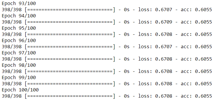
Here you can see that we higher loss and less accuracy.
Evaluation:
The model’s evaluation function. The documentation can be found here https://keras.io/metrics/.
results = model.evaluate(X_test, y_test)

Output:
32/171 [====>.........................] - ETA: 0s
Now we have the results. This object will have 2 metrics Loss and Accuracy.
print(model.metrics_names)     # list of metric names the model is employing
print(results)                 # actual figure of metrics computed
print('loss: ', results[0])
print('accuracy: ', results[1])

Output:
['loss', 'acc']
[0.6395693376050358, 0.6783625724022848]
loss:  0.6395693376050358
accuracy:  0.6783625724022848
To get a clear view about what happened in the whole training process, we can use the object received from model.fit statement. We named it as history.

We can use matplotlib for visualization:
from matplotlib import pyplot as plt

plt.plot(history.history['accuracy'])
plt.plot(history.history['loss'])
plt.legend(['Accuracy', 'Loss'], loc = 'upper left')
plt.show()
If we have added validation split in fit function, we will get both training and validation results.
history = model.fit(X_train, y_train, validation_split = 0.3, epochs = 100, verbose = 0)
plt.plot(history.history['accuracy'])
plt.plot(history.history['val_accuracy'])
plt.legend(['training', 'validation'], loc = 'upper left')
plt.show()
You can see that the validation and training accuracy is not improved in this new model. We used the same training data for validation split also. So the training data was not enough.
Conclusion:
Now you may think that, all that CPU time and GPU time was wasted for less accuracy? Even ML model gave better results!!!
Yes, I too thought the same when I see this accuracy for first time.
We haven’t done one thing yet which is the interesting part of model creation. Yes! Tuning!
This is a base model. We can still tune this model with different number of neurons, layers, epochs, different activation functions, optimizers and loss functions.
Also we can increase the data set to get better results.
I am planning to post an article to tune this model. Will see you in next post.
Thank you for reading our article and hope you enjoyed it. 😊
Like to support? Just click the like button ❤️.
Happy Learning! 👩💻
Nice explanation.. Tks for posting
Thank you Sri.