What is a Hypothesis Testing?
The hypothesis is an assumption which is tested to determine whether the assumption is true or not.
Hypothesis Testing is a process of testing the assumption.
When we do the interpretation, we use statistical methods that provide a confidence or likelihood about the answers. These methods are called statistical hypothesis testing, or significance tests.
How to do Hypothesis Testing?
In Hypothesis testing, the analysts take a random sample of a population and test it to prove the evidence on the acceptance.
The results of this test allows us to explain (interpret) whether the assumption could be true or the assumption has been violated.
When the assumption holds, we call it as Null Hypothesis – Ho.
When the assumption has been violated, we call it as Alternate Hypothesis – H1 or HA.
But now we are confused that which should be considered as Null Hypothesis and which is our alternative.
Null Hypothesis:
The assumption made on the population must be taken as Null Hypothesis.
To be clear about Null Hypothesis, we can say it as: A Null Hypothesis is always going to be a “Status Quo” i.e. “Existing State”.
Example:
- The chocolate manufacturing company’s average production per month is 150 boxes. H0: µ = 150o
- A government official claims that the average dropout rate for local schools is less than 250. H0: µ (Dropout rate) < 250o
- A car dealer’s overall average sales rate per month is minimum 12 cars. H0: µ >= 12
Null Hypothesis assumes that there is no difference from the two mean values.
So, µ = x Sample Mean.
In other words, “No Statistical Significance exists”. (Here significance is the result is unlikely due to chance. So No Significance means, there is no change in the result)
Alternate Hypothesis:
When the Null Hypothesis gets failed, it is obvious that there is a change in mean values. So that shows that observations are the result of a real effect. This is called Alternate Hypothesis.
i.e. Something has changed from the state it was in before the experiment.
Example:
- The chocolate manufacturing company’s average production per month is 150 boxes. H1: µ ≠ 150o
- A government official claims that the average dropout rate for local schools is less than 250. H1: µ (Dropout rate) >= 250o
- A car dealer’s overall average sales rate per month is minimum 12 cars. H1: µ < 12
Example Problem #1:
1,500 women followed the Atkin’s diet for a month. A random sample of 29 women gained an average of 6.7 pounds. Test the hypothesis that the average weight gain per woman for the month was over 5 pounds. The standard deviation for all women in the group was 7.1.
Given:
Population: 1500
Population SD: 7.1
Sample Size: 29
Sample Mean: 6.7 pounds
To test: Test the hypothesis that the average weight gain per woman for the month was over 5 pounds.
So here the average weight gain of the total population is 5 pounds. So population mean is 5 pounds. We need to test the hypothesis that average weight is above 5 pounds.
Obviously our Null hypothesis is µ > 5 pounds.
If we reject the null hypothesis then it means the sample average weight gained is close to or less than the population average weight gained.
i.e. H0: µ > 5
As H0 > 5, our alternate hypothesis is the opposite of Null Hypothesis.
Here H1 <= 5
Example Problem #2:
Using this example, lets learn more about critical region, One Tail Test & Two Tail Test.
The average intelligence of a School’s students is less than or equal to 100 with a standard deviation of 15.
A new staff at this school claims that the students in this school are above average intelligence. A random sample of thirty students IQ scores have a mean score of 112. Is there sufficient evidence to support the new staff’s claim?
H0: µ <= 100
H1: µ > 100
If the Null Hypothesis is to test the population mean is greater than some value or less than some value, then we need to test the hypothesis to find whether the sample mean is falling under the area greater than the population mean or less than the population mean. In this case you are considering the one direction under the normal curve.
A one-tailed test is where you are only interested in one direction.
If a mean is 100, you might want to know if a set of results is more than 100 or less than 100.
If the sample mean is 112.5 then it should be in somewhere right side (positive) from the mean.
Finding the rejection region:
From the above Students example, the Null Hypothesis is <= 100.
So as per the Null Hypothesis all the IQ values are falling below the mean (=100) of the Normal curve.
Now we need to know at what percentage of confidence level we need to do this test? If it is not given then by default 95% confidence level. If the confidence level is 95% then the significance level is 100-95 = 5%
As we consider the region under the normal curve is unit.
C (confidence value) = 0.95
α (Significance value) = 1-0.95 = 0.5
One Tail Test:
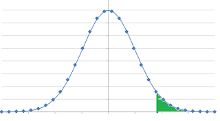
If the value falls under the 0.05 area of the right side of the normal curve then the null hypothesis fails. So the rejection region is in right side. If the rejection region is in right side then it is called the right tail or upper tail.
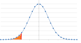
If the H0 >= 100 & H1 <100 then we reject the Null Hypothesis if the value falls under 100. So now the rejection region is in left side of the mean which is called left tail or lower tail.
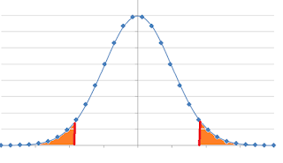
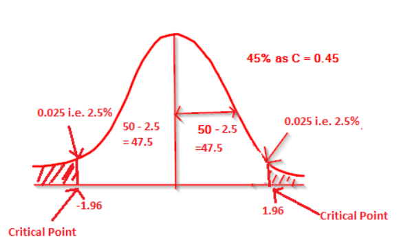
Two Tail Test:
If the Null hypothesis is H0 = 100, then the area where all the 95% of confidence level lies between both the tails (by the empirical rule).
Now the Null hypothesis should lie in this region and not in the left most area or in the right most area.
At this time we split the 0.05 significance level by 2.0.05/2 = 0.025.
Now the rejection region would be in both the sides and so it is a two tailed test.
Assumptions:
If the level of confidence is not given then it is 95%. i.e. 0.95Ie. α (Level of significance) = 1-0.95 = 0.05Why we need to subtract from 1?
As the normal distribution is a continuous probability distribution, the sum of all the possibilities (both success (confidence – C) and failure (significance – 𝛂) is 1).
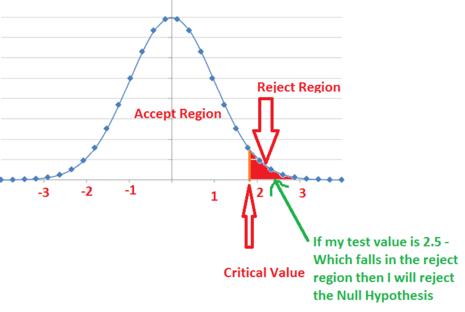
Critical Value/Point:
The value lies in the line that separates the accept region and reject region is taken as critical value.
But How to find the critical value?
Critical values will be calculated from alpha levels.
If the Confidence Level is 95% and then the C value will be 0.95.
Then alpha value becomes 1-0.95 = 0.05
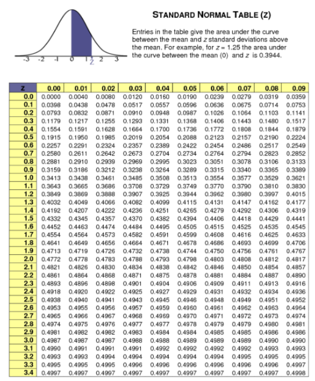
If we look up the value for 0.45 in the z table values not in the left most column and top most row, it is from the values lies in the z table.
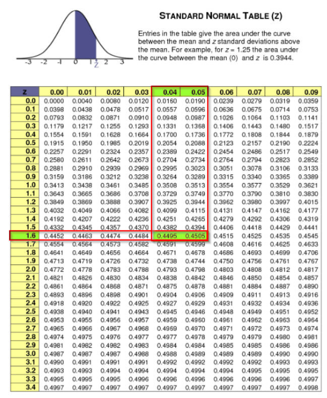
Z table:
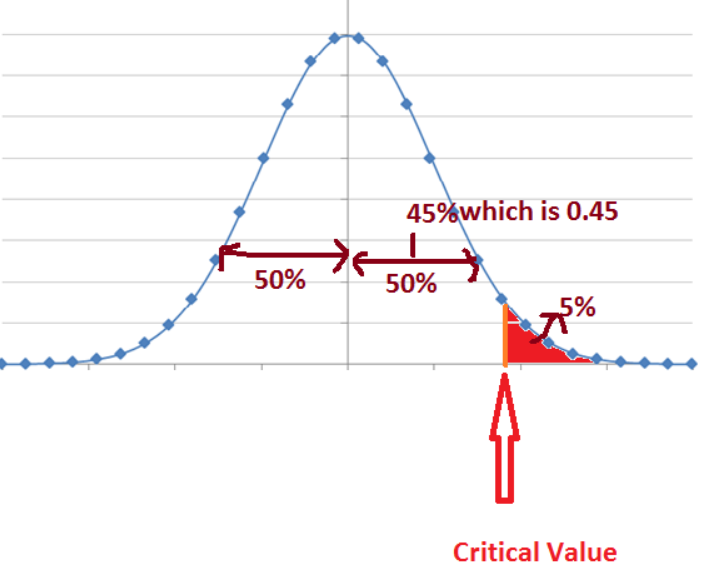
Per the below picture, entire area from the mean to the right most end of normal curve is 50%.
If the test is right tail and accept region is in left, then the rejection region is 5% area in the right most end of the normal curve (shaded region in the below distribution).
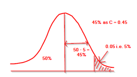
If we remove the shaded region then we have 45% of area in right side. i.e. 0.45
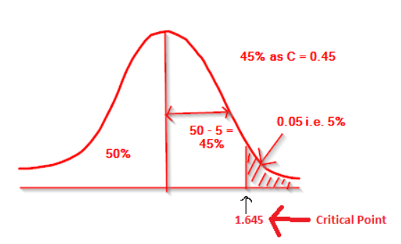
In the below table, if you look for 0.45 nearby value, we can see two values 0.4495 when we round this value it is 0.45. Also we can see the value 0.4505. If we take both these values in account, then the row and column values are added and we get 1.6 from left and 0.04 & 0.05 from top. So we get z value as 1.645.
So for one tailed test, if the confidence level is 95% then its z value is 1.645.
If it is a two tailed test, then the rejection region will be split into two halves. So the rejection region will be 0.05/2 = 0.25.
So the acceptance region will be 50-2.5 = 47.5
i.e. C value is 0.475.In the same way as we look z value for 95%, in the z table, we can find the value near to 0.475.
We get the exact value 0.4750. Its corresponding z value is 1.9 from left & 0.06 from top. So 1.96.
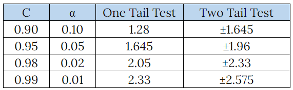
This z value will always be same for the normal distribution for the percentages. So practically we do not need to calculate each time we need to find the critical point. For the most frequently used Confidence levels, below are the z values.
Learn More about Inferential Statistics & Hypothesis Testing:
Conclusion:
In this article, we learned about Hypothesis Testing, One tailed & Two tailed testing with examples.
In next article, we will learn about how to do these testing.
Thank you! 👍 Happy Learning 🎈.
Like to support? Just click the heart icon ❤️.